1 Model framework
VALUE simulates half-hourly electricity-system operation and annual changes in its assets. Generation, storage and imported electricity enter market clearing through offers. Annual asset income, operating cost and expansion headroom determine investment and retirement proposals. Development times and regional success rates determine when projects enter the operating fleet. Outputs include generation, storage charging and discharging, electricity shortfall, prices, system cost, carbon emissions and operating capacity by technology.
Time, units and space
The operating interval is half an hour in UTC. Each model year has 365 days and 17,520 intervals, with 28 days in February. Power is measured in MW and interval energy in MWh: 1 MW supplies 0.5 MWh in a half-hour. A complete operating year supplies the annual investment calculation; commissioning and retirement update the fleet between years.
The national single-node model clears aggregate demand and supply in Great Britain, with interconnectors offering external electricity. The zonal model forms an electricity balance for each zone from resource locations and demand shares, subject to line and boundary constraints. Chapter 7 specifies the 23-zone inputs, resource allocation, network constraints and numerical solution.
Monetary calculations use constant start-year prices as a scenario convention, with 2025 as the default start year. Input tables retain the price years of technology costs, imported electricity and policy parameters. Chapter 2 lists the inputs and conversions; Chapter 5 gives generator restart costs in 2025 GBP.
Operating methods
Default national operation uses the value-corrected configuration and value-bid-at-cost-psm module. Its Native kernel uses native-corrected-v1 to determine offer ordering, uniform marginal settlement, storage operation and thermal downward adjustments. Each period first schedules supply against forecast demand and availability, then balances realised demand and availability using the remaining flexibility. Chapter 5 develops the algorithm in this order.
value-staged-bid-at-cost-psm passes the national schedule to a separate balancing module. value-copperplate-balancing calculates single-node balancing, while value-zonal-redispatch-balancing calculates zonal redispatch subject to network constraints. Chapter 4 connects scheduling, balancing and storage state; Chapter 7 defines the zonal objective functions, constraints and settlement.
Perfect-foresight dispatch uses the complete demand and availability sequences within its solution window to optimise generation, imports and storage jointly. Chapter 8 defines the objective, time-coupled constraints and terminal storage condition of value-perfect-foresight-lp. It also specifies the run-of-river and reservoir calculations from natural inflows to available hydroelectricity.
Initial conditions and annual sequence
A calculation is defined by its input data pack, start and end years, selected modules and numerical parameters. native_initial_state constructs initial_state from the fleet, REPD projects, costs, development timelines and regional success rates. Operating assets carry technology, region, power capacity, storage energy capacity, costs and lifetime. Planned projects carry capacity, status and expected commissioning year. Chapter 2 specifies the input fields, values and initialisation rules.
Each year advances the planning projects, operates the annual market and constructs the following year's assets and projects. AnnualModelOrchestratorV2.run calls the modules in the order below. The corresponding chapters develop each calculation, including its equations, initial values and boundary conditions.
| Order | Calculation | Variables and functions | Chapter |
|---|---|---|---|
| 1 | Update the operating fleet from project commissioning years | planning.advance_year produces advanced.operating_state |
6 |
| 2 | Prepare demand, weather, availability and external exchange | psm_input_factory produces model_input |
2, 3 |
| 3 | Clear operating periods and aggregate their results | psm.run produces market |
4, 5, 7, 8 |
| 4 | Calculate expansion headroom from annual demand, availability and storage use | policy.evaluate produces headroom |
6 |
| 5 | Evaluate income by owner and technology-region group | adapt_market_for_investment assembles accounts; investment.decide produces decision.proposals |
6 |
| 6 | Admit investment projects using development times and success rates | planning.admit_projects produces admission |
6 |
| 7 | Update asset age, retirement and new projects | transition.apply produces next_state |
6 |
Storage inventory updates within operating periods, while cost observations update annually. National operation creates storage objects for each operating year. The previous year's sold energy and dwell time enter the following year's dynamic storage cost. Chapters 4 and 5 specify opening inventory, efficiencies, self-discharge, period power limits and year-end treatment.
Annual investment uses realised income, total capital expenditure, target payback and preferred return. Gas and biomass investment income deducts operating costs; wind, solar and storage use revenue to calculate investment returns. Chapter 6 gives the cost components, four decision tiers, development times, success rates and asset-update pseudocode.
Annual outputs sum period results or weight them by electricity volumes. Served energy equals demand less unserved energy, system cost aggregates operating and annualised capital expenditure, and carbon accounting uses generation, imported electricity and equipment capacity. Chapters 5, 6 and 9 define these quantities, their units and denominators.
Back to contents ↑2 Initial data and input processing
VALUE constructs an electricity-system study from demand, weather, operating assets, planned projects, technology parameters and external-market prices and flow limits. Source years identify the observed samples; the study's start year selects the operating fleet and the subsequent investment calendar. The default value-corrected configuration reads the following public2 packages, available from the data page.
| Study inputs | Package | Contents |
|---|---|---|
| Great Britain, national | value-uk-open-data-pack-public2 |
Demand, representative-point weather, fleet, planning, costs and five external markets |
| Great Britain, 2025–2034 with calendar-mean weather | value-uk-calendar-vx-trade001-public2 |
R029 configuration with 2022 demand and 2020–2024 weather |
| Great Britain, 23 zones | value-uk-research-suite-v1-public2 |
National inputs, zonal demand, asset allocation, corridors and external boundaries |
| VALUE 101 | Synthetic teaching inputs | 2025–2026 studies with a full 17,520-period year and a 48-period exercise; generation rules are given below |
Input roles connect files to physical quantities. The package's manifest.json binds each role to its file and declares its column, unit and temporal resolution. The following table gives the R029 filenames and the variables supplied to the calculations.
| Input role | Main data or fields | Computational use |
|---|---|---|
| Actual and forecast demand | demand_mw in actual_mw.csv; forecast_mw in forecast_mw.csv |
Real-time balancing, day-ahead clearing and demand error |
| Fleet and initial assets | fleet.json, annual operating_state |
Technology parameters, representative locations and dispatch capacities |
| Projects and planning | repd_projects_normalized.csv, regional_technology_success_rates.csv, planning_timelines.json |
Initial operational assets, project success rates and stage durations |
| Weather | calendar_mean_solar_2020_2024.nc, calendar_mean_wind_2020_2024.nc |
Available wind and solar generation at representative points |
| Technology-average profiles | sa.csv, wa.csv, we.csv |
Technology-average investment inputs for solar, onshore wind and offshore wind |
| Capital and policy | capital_costs.json, model_parameters.json, mechansim cost.xlsx |
Investment costs, financial parameters and policy expenditure |
| External markets | Country-specific flow_mw, price_gbp_per_mwh |
Available interconnector exchanges and external offers |
| Zonal network | Zones, corridors, boundaries, asset mapping and zonal demand | Spatial supply–demand balance and transmission constraints |
Model clock and units
The operating year contains 17,520 half-hours on a 365-day UTC calendar. Period zero starts at 00:00 on 1 January; February contains 28 days. Asset capacity is measured in MW, stored energy in MWh, money in GBP and electricity price in GBP/MWh. The period_start_utc function assigns each period its calendar time.
Demand enters as power in MW. The default national algorithm passes the values from read_role through _kernel_inputs to run_simulation in MW. The staged and optimisation interfaces use build_chronology in canonical_psm_data to form period energy: series["demand.real"].values and series["demand.forecast"].values hold MW, while demand and forecast_demand hold MWh per period. With zero-based period index t,

Annual demand energy is the sum of demand. A user-supplied column expressed in MWh per source period is divided by that period's duration in hours to obtain MW before half-hour alignment. VALUE 101 writes its synthetic power values under the column name mwh; those values enter the same MW-to-MWh calculation above.
Column selection, missing values and annual alignment
Time-series loading follows the declared column and header. read_series uses csv_column with csv_header=true; each cell in that column must be numeric and finite. An empty sequence, a missing named column or an invalid numeric cell terminates loading. For a file with an inferred column, an integer sequence of at least three values increasing by one requires an explicit column declaration.
Header and column inference follow the contents of the file. A declared csv_header takes precedence. Otherwise the first row is a header when it has at least one populated cell and every populated cell is non-numeric. With a missing csv_column, strict reading selects the sole wholly numeric column; multiple numeric columns require an explicit selection. The user-workspace reader selects the first wholly numeric column in an ambiguous file. Declaring the column fixes this choice independently of column order.
Hourly inputs are expanded before the requested run window is selected. align_clock reads interval_minutes=60 as two copies of each source value and interval_minutes=30 as one value per half-hour. With an absent interval declaration, lengths of 8,760 and 8,784 identify hourly years. Other declared resolutions terminate loading. The hourly conversion is applied once.
Leap-year demand retains its annual energy on the 365-day model clock. After hourly expansion, a 17,568-period year loses the 48 values beginning at (31 + 28) * 48, corresponding to 29 February. In normalize_half_hour_year, numbers contains the source values and reduced the retained values. For a positive retained sum,

An all-zero demand series remains zero. A zero retained sum with a positive original sum terminates conversion. Other time-series roles remove the same 48 values and retain the remaining values. An explicit leap_policy="keep" retains the source calendar and selects the required leading periods.
The run consumes the first periods values of a sufficiently long aligned sequence. A shorter series repeats from its beginning when cyclic=true, or when its role supplies the cycling convention; external-market flows and prices have this convention. Strict package reading requires that declaration for shorter demand or investment sequences. User-workspace reading fills a short series by repetition. These rules determine the numerical input for a partial-year or full-year run.
The following sequence produces the aligned values. path is the bound file, spec contains its declarations, policy.strictness selects strict package reading or user-workspace reading, and cyclic is the role's repetition default.
read = read_series(path, spec, mode="declared-v2", strictness=policy.strictness)
values = align_clock(read.values, periods, spec, mode="declared-v2",
                     strictness=policy.strictness, cyclic_default=cyclic)
return values
Observed demand and missing settlement periods
The supplied GB demand shape uses NESO's 2022 half-hour actual demand and day-ahead forecast. Each of actual_mw.csv and forecast_mw.csv contains 17,520 values after UTC preprocessing. Each subsequent model year uses the same aligned 2022 actual-demand and forecast-demand sequences. Their power and energy totals are
| Series | Minimum power MW | Maximum power MW | Mean power MW | Annual energy MWh |
|---|---|---|---|---|
| Actual demand | 15,080 | 46,042 | 26,587.967637 | 232,910,596.5 |
| Day-ahead forecast | 14,240 | 46,760 | 26,611.131963 | 233,113,516 |
Demand preprocessing resolves settlement records before interpolation. Rows with the same settlement date and settlement period are ordered by publication time; the latest publication is retained, with the final row breaking a tie. UK local settlement times are then placed on the UTC half-hour axis. The 17,518 source rows yield 17,516 distinct periods, leaving four missing half-hours.
Missing demand periods are filled by linear interpolation between their adjacent known values. One missing period receives the mean of the endpoints. Two consecutive missing periods receive one-third and two-thirds of the endpoint difference added to the preceding value. The four replacements in the 2022 input occur on 30 October:
| UTC time | Forecast demand MW | Actual demand MW |
|---|---|---|
| 2022-10-30 09:00 | 22,638.666667 | 24,649 |
| 2022-10-30 09:30 | 22,899.333333 | 24,727 |
| 2022-10-30 23:00 | 19,063.333333 | 20,494.666667 |
| 2022-10-30 23:30 | 19,086.666667 | 19,689.333333 |
User demand timestamps are converted to UTC before the same model-year alignment. The mapping accepts UTC or Europe/London and a declared DD/MM/YYYY or MM/DD/YYYY date order. Timestamps must identify a strictly increasing sequence with a regular 30- or 60-minute step; duplicates, unresolved dates and gaps terminate mapping. The resulting row order is placed from 1 January 00:00 UTC in each model year, retaining the input's sequence of weekday and holiday effects.
Initial operating assets
The initial renewable and battery stock is selected from the DESNZ Renewable Energy Planning Database, second quarter 2025, released in July. Its 12,977 project rows and 53 source fields yield 10,653 rows and 14 fields after technology and positive-capacity filtering. normalize_repd retains onshore wind, offshore wind, solar, battery and gas technologies; capacity_mw, x_coordinate and y_coordinate are converted to numbers, with failed conversions stored as missing values.
The normalised project table retains the information needed for date and location selection. Its fields are project_id, site_name, technology, technology_source, capacity_mw, development_status, region, country, planning_application_submitted, planning_permission_granted, under_construction, operational, x_coordinate and y_coordinate. Date strings remain available for the asset and planning readers to parse.
Operating wind, solar and battery capacity requires Operational status, a readable operational date at or before the study's start year, and positive installed MW. build_repd_operational_snapshot parses the date with day-first order and skips records with missing dates or invalid capacity. Solar and onshore projects first use the region-to-city mapping in Chapter 3. Remaining projects use geographic coordinates and the nearest representative of their technology; OSGB coordinates are converted from EPSG:27700 to EPSG:4326 when required. A project with neither a regional assignment nor usable coordinates contributes zero to the mapped initial wind or solar stock.
Initial battery MW is distributed among the storage entries other than pumped hydro. For each entry, weighted[asset_id] equals the larger of its pool_limit and 1; weight_total is their sum. native_initial_state assigns capacity = operational_storage_mw * weighted[asset_id] / weight_total. Its energy is capacity * duration, where duration comes from the technology catalogue. The 2025 pumped-hydro stock is specified separately as 2,828 MW and 26,700 MWh.
The R029 2025 stock contains the capacities below. Its aggregated nuclear availability is 0.723, and run-of-river generation uses 0.3487 multiplied by the seasonal shape in Chapter 5. GBP1 selects its nuclear units through the station schedule, with the station availability and retirement rules also defined in Chapter 5.
| Technology | Asset rows | Power MW | Stored energy MWh |
|---|---|---|---|
| Combined-cycle gas turbine CCGT | 1 | 28,000 | — |
| Run-of-river hydro | 1 | 2,000 | — |
| Nuclear | 1 | 5,958 | — |
| Open-cycle gas turbine OCGT | 1 | 4,146 | — |
| Biomass and waste | 1 | 4,762 | — |
| Offshore wind | 18 | 14,679 | — |
| Onshore wind | 11 | 14,711.65 | — |
| Solar | 11 | 10,066.98 | — |
| 0.25C battery | 1 | 299.984165 | 1,199.936659 |
| 0.5C battery | 1 | 2,465.869834 | 4,931.739667 |
| 1C battery | 1 | 74.996041 | 74.996041 |
| Hydrogen storage | 1 | 0.749960 | 187.490103 |
| Pumped hydro | 1 | 2,828 | 26,700 |
Planning inputs
Project development uses technology- and region-specific success rates and technology-specific stage durations. regional_technology_success_rates.csv contains 46 records; planning_timelines.json supplies durations in months. development_stage_timelines, repd_status_to_timeline and success_rates are stored in the initial state and supply both existing planned projects and new investment proposals.
The input medians distinguish development from construction. Status mappings select the relevant remaining stages. The following preprocessing constructs the initial project list; Chapter 6 advances these projects and admits new investment proposals each year.
| Technology | Median development months | Median construction months |
|---|---|---|
| Solar | 27.8 | 4.9 |
| Onshore wind | 62.5 | 15.0 |
| Offshore wind | 110.1 | 32.2 |
| Battery | 31.3 | 10.1 |
Initial planned projects are selected by capacity, development status and recorded progress. native_initial_state uses the controls below; the default planning.success_mode="expected" is read as success_mode="expected_capacity". year is the study's start year and capacity is the source project's MW.
| Parameter | Default | Use |
|---|---|---|
planning.minimum_project_size_mw |
1 MW | Smallest positive project admitted |
planning.include_uncertain_projects |
true |
Admit application, appeal and revised statuses |
planning.zombie_filter_enabled |
true |
Apply status, progress and construction-overrun filters |
planning.zombie_status_stale_year |
2015 | Latest-progress cutoff for uncertain projects |
planning.construction_grace_years |
2 years | Added to the estimated construction completion year |
planning.max_completion_year |
2040 | Latest admitted completion year |
planning.timeline_statistic |
median |
Select median or mean stage durations |
planning.defer_spread_years |
3 years | Maximum added delay for inferred completion dates |
planning.random_seed |
0 | Input to project-specific success draws |
planning.repd_battery_assignment |
value_proportional_split |
Allocate generic battery capacity among four storage technologies |
A replacement application supersedes its older project record. The preprocessing reads Ref ID and Are they re-applying (New REPD Ref) in the raw REPD table and excludes the old record when the replacement is a different, non-empty identifier present in that table. It also excludes capacity below minimum_size and non-positive or unparseable capacity.
Development-status filtering acts on stripped, lower-case labels. terminal_statuses always excludes operational, abandoned, planning permission refused and application withdrawn. With zombie_filter=true, the additional excluded labels are application refused, appeal refused, appeal withdrawn, decommissioned, application expired and finished. Setting include_uncertain=false retains only under construction, awaiting construction and planning permission granted.
The recorded progress cutoff applies to application submitted, appeal lodged and revised. _date_year extracts the first four-digit year beginning with 19 or 20 from each date string; a missing year yields None. latest_progress_year takes the latest known year across planning_application_submitted, planning_permission_granted, under_construction and operational. With the progress filter enabled, an uncertain project is excluded when this year is at or before zombie_stale_year; a missing progress year passes this particular filter.
The completion year first uses a recorded future year and otherwise uses the remaining stage duration. timeline_months(source_technology, status) selects timeline_type from repd_status_to_timeline, replaces its mean or median suffix with timeline_statistic, and reads the selected technology entry in development_stage_timelines. A missing status mapping selects total_median by default; a missing stage entry uses development_timelines, with a final fallback of 12 months. Storage components use the battery duration table.
The inferred completion date adds a deterministic delay of zero to defer_spread_years whole years. The following sequence uses the source project_id to calculate that delay; an existing future date bypasses the duration and delay calculations.
completion = next((candidate for candidate in (
    _date_year(row.get("operational")),
    _date_year(row.get("under_construction")),
) if candidate is not None and candidate > year), None)
if completion is None:
    months = timeline_months(source_technology, status)
    completion = year + max(1, int(math.ceil(months / 12.0)))
    if defer_spread_years > 0:
        completion += int(
            hashlib.sha256(project_id.encode("utf-8")).hexdigest()[:8], 16
        ) % (defer_spread_years + 1)
Construction status receives a separate elapsed-time check. For under construction with a known construction_year, preprocessing forms construction_end = construction_year + max(1, math.ceil(timeline_months(source_technology, status) / 12)) + construction_grace. With zombie_filter=true, a value earlier than year excludes the project. A completion later than maximum_completion also excludes the project.
Initial project success uses a technology–region lookup. _planning_probability reads technology, region and success_rate, clamps each readable rate to [0,1] and skips unreadable rates. A missing required column yields an empty rate table. The lookup first uses the project's lower-case region, then the technology's gb entry, then 1.0. The calculation below gives probability, the dimensionless draw draw, and the admitted capacity; all components of one physical battery project share its draw.
probability_key = "battery" if source_technology == "battery" else _technology(source_technology)
probability = success_rates.get(
    (probability_key, region.strip().lower()),
    success_rates.get((probability_key, "gb"), 1.0),
)
draw = int(
    hashlib.sha256(f"{random_seed}:{project_id}".encode("utf-8")).hexdigest()[:13], 16
) / float(16 ** 13 - 1)
realised_failure = success_mode == "seeded_stochastic" and draw > probability
components = typed_project_components(project_id, source_technology, capacity)
for component_id, technology, declared_component_capacity, assignment_method in components:
    effective_capacity = (
        declared_component_capacity * probability
        if success_mode == "expected_capacity" else declared_component_capacity
    )
Generic battery projects are split before their success-adjusted capacities are recorded. typed_project_components uses scheme_c_storage_weights, formed from the same positive fleet weights used for initial battery stock, to allocate source MW among 1c_battery, 0.5c_battery, 0.25c_battery and hydrogen_battery. Each declared_component_capacity equals the source capacity times its weight divided by total weight. The settings all_1c, all_0.5c and all_0.25c assign the full capacity to one technology; exclude_untyped removes generic battery projects from the initial list. Projects with a specified technology retain that technology and capacity.
The expected-capacity mode multiplies each component's declared MW by its success probability. The stochastic setting planning.success_mode="stochastic", read as seeded_stochastic, retains full declared MW and sets phase="failed" and outcome="failed_planning" when draw > probability; equality passes. Successful projects and expected-capacity projects receive phase="active" and outcome="active". Storage energy is effective_capacity * duration_hours in MWh. PlanningProject stores these values with expected_completion_year=completion, the start year, status, technology and region for Chapter 6's annual progression.
New investment proposals use the success-rate lookup in endogenous_planning._success_rate. It selects the regional rate, then the technology's regional mean, then 0.75. Chapter 6 defines proposal capacity and the subsequent planning process.
Capital costs and storage parameters
Capital costs, target returns and payback periods are supplied as distinct financial inputs. The R029 configuration reads capital_costs.json and model_parameters.json; the capital-cost material draws on BEIS Electricity Generation Costs 2020 and Arup. The table gives the financial parameters assigned to the initial assets. Annual capital recovery uses capital_discount_rate=0.05; the investment calculations and effective decision thresholds are defined in Chapter 6.
| Technology | Capital cost GBP/MW | preferred_rate |
Target payback years |
|---|---|---|---|
| Solar | 659,000 | 0.076 | 25 |
| Onshore wind | 1,588,000 | 0.076 | 30 |
| Offshore wind | 3,976,000 | 0.089 | 30 |
| CCGT / OCGT | 2,400,000 | 0.089 | 25 |
| Biomass and waste | 1,500,000 | 0.089 | 25 |
| 1C battery | 330,000 | 0.0825 | 10 |
| 0.5C battery | 350,000 | 0.165 | 10 |
| 0.25C battery | 415,000 | 0.0825 | 10 |
| Hydrogen storage | 600,000 | 0.01375 | 25 (default) |
Storage energy losses follow separate charging and discharging efficiencies. Round-trip efficiency is charge_efficiency * discharge_efficiency, giving  for the 0.5C battery. The catalogue also supplies duration, economic lifetime and
maximum_cycles. These values enter the storage-state and cost equations in Chapters 4 and 6; initial stored energy is specified with the operating algorithm in Chapter 4.
| Technology | Catalogue duration h | Charging efficiency | Discharging efficiency | Catalogue economic life years | Cycle parameter maximum_cycles |
|---|---|---|---|---|---|
| Pumped hydro | 4 | 0.87 | 0.87 | 30 | 1,000,000 |
| 1C battery | 1 | 0.81 | 0.81 | 15 | 3,000 |
| 0.5C battery | 2 | 0.98 | 0.98 | 15 | 5,000 |
| 0.25C battery | 4 | 0.81 | 0.81 | 15 | 8,000 |
| Hydrogen storage | 250 | 0.57 | 0.57 | 10 | 1,000 |
Source price years remain attached to the numerical inputs. Storage costs and policy budgets are expressed in 2025 GBP; BEIS capital-cost inputs retain 2020 values, the European electricity samples retain their 2022 or 2021 values after currency conversion, and nuclear-policy entries carry their declared 2015 or 2024 price years. Restart costs use the conversion in Chapter 5. The currency reader converts euros to pounds using eur_per_gbp.
Annual policy spending uses the schedules in mechansim cost.xlsx. The workbook combines NESO Capacity Market and balancing-cost series, Ofgem RO/FIT/REGO material and LCCC CfD data. Chapter 6 specifies how these inputs enter annual accounts.
External markets and zonal demand
External electricity exchange is limited by a time-varying envelope and priced by the corresponding foreign market. R029 supplies 17,520-row files for France, Belgium, the Netherlands, Norway and Ireland. Each file provides flow_mw and price_gbp_per_mwh alongside its period and source timestamps. NESO line names associate NEMO_FLOW with Belgium, BRITNED_FLOW with the Netherlands and NSL_FLOW with Norway.
Foreign prices use Ember's compilation of ENTSO-E day-ahead prices. France, Belgium, the Netherlands and Norway use 2022; Ireland uses 2021. An hourly EUR/MWh value is divided by 1.1 EUR/GBP and assigned to both receiving half-hours. Negative prices retain their sign. R029 stores the converted GBP/MWh values; a GBP1 file such as Belgium_price.csv supplies Price (EUR/MWhe) and receives the same conversion through read_series.
The positive and negative values of flow_mw define import and export capacity, respectively. Multiplication by period_hours yields signed period energy raw_availability, from which the two non-negative envelopes are calculated:

The default national market offers imports in day-ahead clearing. Chapter 5 defines their use during clearing and balancing, and Chapter 7 applies the external-boundary capacities in the zonal model. The R029 envelope ranges and mean prices are
| Boundary | Flow range MW | Price year | Mean price GBP/MWh |
|---|---|---|---|
| Belgium | −1,022 to 1,020 | 2022 | 222.292608 |
| France | −3,091 to 2,997 | 2022 | 250.789325 |
| Ireland | −987 to 998 | 2021 | 123.937076 |
| Netherlands | −1,076 to 1,062 | 2022 | 219.917959 |
| Norway | −1,263 to 1,399 | 2022 | 126.503575 |
Zonal demand uses the national study's total and the network input's spatial shares. align_zonal_demand matches network and study period_ids, which must be unique and have corresponding records. Actual and forecast input energy must be finite, non-negative and equal in length to the period list. In scenario_scaled_zonal_shares, output_real holds the study's actual MWh and network_national the network's national MWh at index:

The final zone receives the remaining national energy after the preceding zones have been assigned. If both national inputs equal zero, scale=1.0; positive study demand with zero network national demand terminates alignment. The following sequence gives the complete allocation, with zone_ids retaining the network's declared order:
aligned = {zone_id: [] for zone_id in zone_ids}
for index, period_id in enumerate(periods):
    network_national = network_national_mwh[index]
    if network_national == 0.0 and output_real[index] == 0.0:
        scale = 1.0
    elif network_national == 0.0:
        raise ValueError("Zonal demand requires positive network national demand")
    else:
        scale = output_real[index] / network_national
    remaining = output_real[index]
    for zone_id in zone_ids[:-1]:
        value = network_demand_mwh_by_zone[zone_id][index] * scale
        aligned[zone_id].append(value)
        remaining -= value
    aligned[zone_ids[-1]].append(remaining)
The alternative network_pack_absolute_demand sets output_real to network_national_mwh and scale=1.0. Its forecast is output_real[index] * forecast[index] / real[index]. When real[index] is zero, both forecast[index] and output_real[index] must also be zero and the resulting forecast is zero. The same final-zone remainder rule preserves the national energy total.
VALUE 101 synthetic inputs
VALUE 101 supplies deterministic demand, weather and investment profiles. _demand returns MW for zero-based half-hour index period; day and hour identify its day and hour. weekday equals 1 when day % 7 < 5 and 0.92 otherwise. teaching_peak is 30 MW at period % 48 == 31 on days 0 and 182, and zero elsewhere:
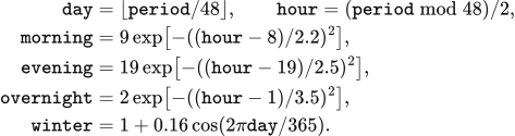

The day-ahead forecast is _demand(period) + balancing_margin, rounded to six decimal places. balancing_margin is 12 MW at period % 48 == 30 on days 0 and 182, and zero elsewhere. The 12 MW addition precedes each of the two actual demand peaks by half an hour.
The solar investment coefficient multiplies daylight and seasonal terms. _solar_profile returns zero for hour < 6 or hour > 18. During the daylight window it uses the same day and hour definitions:

The wind investment coefficient combines daily, 29-day and annual components. _wind_profile limits the result to 0.08–0.92 and rounds it to six decimal places:
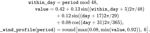
The offshore investment coefficient is 1.08 times _wind_profile(period), capped at 1 and rounded to six decimal places. Solar, onshore and offshore arrays are bound to profiles.vre_solar, profiles.vre_onshore and profiles.vre_offshore.
The synthetic weather grid has one point at 52°N, 0°E and 8,760 hourly samples. Here hour is the zero-based hourly index through the year; hourly_solar is accumulated radiation in J/m² and hourly_wind is wind speed in m/s:

Dispatch converts this wind speed through the wind curve and this solar series through the instantaneous-input rule in Chapter 3. Investment uses the coefficients above. The French boundary supplies a constant 12 MW import envelope and 82 GBP/MWh price; the other four boundaries have zero exchange capacity and a price input of 200 GBP/MWh. build_value_101_packs writes these sequences into the teaching inputs.
3 Weather and available generation
Wind and solar availability is calculated for each asset from its installed capacity and the weather assigned to its representative location. capacity_mw is installed MW, availability is the dimensionless weather conversion coefficient, available_mw is available power, and available_mwh is energy available in one operating period:

The weather calculation produces an upper supply limit for clearing. Dispatch determines the accepted energy in Chapters 4, 5 and 7. Annual investment uses the technology-average profiles described at the end of this chapter and the capacity limits in Chapter 6.
Weather inputs and spatial sampling
R029 represents each calendar hour by the mean of the 2020–2024 ERA5 observations for that month, day and hour. The source contains 43,848 hourly records. Removing the two leap days removes 48 hours, leaving five observations for each of 8,760 retained calendar hours. The resulting annual sequence is reused in each model year.
Wind speed is averaged after calculation of the vector magnitude at each source hour. The preprocessing first takes the square root of u100 squared plus v100 squared, then forms its calendar mean as wind_speed; it also retains u100 and v100. The solar file contains accumulated downward horizontal radiation ssrd. The R029 files are calendar_mean_wind_2020_2024.nc and calendar_mean_solar_2020_2024.nc.
The weather grid covers Great Britain and adjacent seas at 0.25° resolution. The files have the following coordinate extents and array sizes:
| Input | Latitude range | Longitude range | Latitude × longitude × day × hour |
|---|---|---|---|
| Solar radiation | 45°–65°N | 14°W–4°E | 81 × 73 × 365 × 24 |
| 100 m wind | 46°–65°N | 14°W–5°E | 77 × 77 × 365 × 24 |
A representative site receives the nearest grid latitude and longitude. In point_series, site coordinates latitude and longitude and grid arrays lats and lons are in degrees. lat_index and lon_index select the smallest absolute coordinate differences; a tie selects the first grid-array entry:

Spatial extraction accepts latitude–longitude–day–hour arrays and time–latitude–longitude arrays. The selected point is flattened in source order to an hourly sequence. An empty sequence, masked value, non-finite value or other array layout terminates weather loading. Each site's lat and lon are supplied by fleet.locations; representative_sites matches those locations to the generator names in fleet.json.
Hourly weather and half-hour dispatch
Weather values are assigned according to the physical meaning of their timestamps. The default weather method has clock="v2". A binding's time_convention takes precedence; otherwise GRIB_stepType="accum" denotes an accumulation ending at the timestamp, and other fields use the instantaneous convention. hour_index maps zero-based half-hour index t to source index index, wrapping after hours source values:

An hourly accumulation ending at 01:00 supplies the periods beginning at 00:00 and 00:30. The instantaneous rule assigns the sample at 00:00 to the period beginning at 00:00, and the sample at 01:00 to the periods beginning at 00:30 and 01:00. Solar geometry is evaluated at each receiving period's midpoint.
The R029 calendar-mean files declare instantaneous inputs, so they use the second row of the index rule. The supported clock="v1" setting instead uses index = (t // 2) % hours: each source value serves two consecutive half-hours. These index rules apply to the declared source order, including the wrap from the final source hour to the first.
Wind power curve and losses
Wind availability follows a cut-in speed of 3 m/s, cubic growth to rated output, constant rated output and a cut-out limit. hourly_unit_cf reads wind_speed when that variable is present; otherwise it forms the magnitude from u100 and v100. wind_unit_output uses a 20-unit output scale and its result is divided by 20 to obtain the dimensionless hourly coefficient hourly. For speed speed, rated speed rated and cut-out speed cut_out, all in m/s,

Onshore wind uses rated=9.7 and cut_out=25; offshore wind uses rated=10.5 and cut_out=30. Output equals the rated value at the cut-out speed and falls to zero above it. The cubic segment is bounded to the 0–20 range before conversion to hourly.
The delivered wind coefficient multiplies the assigned hourly[index] by the product of wake, energy-availability and electrical factors. method.multiplier(technology) reads the following values from value_uk_vre_loss_factors_v1.json when loss_factors=true, the default setting:
| Technology | Wake factor | Energy-availability factor | Electrical factor | multiplier |
|---|---|---|---|---|
| Onshore wind | 0.95 | 0.97 | 0.98 | 0.90307 |
| Offshore wind | 0.88 | 0.945 | 0.98 | 0.814968 |
At 8 m/s the onshore curve gives 0.5476061707. Multiplication by 0.90307 gives approximately 0.49453, corresponding to 49.453 MW of available power from 100 MW of installed capacity. The supported setting loss_factors=false sets multiplier=1.0 and uses the curve output directly.
Horizontal radiation and solar conversion
Solar conversion first expresses each source-hour radiation value as irradiance. hourly_unit_cf reads ssrd as raw in J/m² and returns hourly in kW/m². The input filter and unit conversion are

The default solar method uses plane_of_array=true and a performance ratio of 0.83. Array-plane conversion applies when clock="v2" and time_convention="accumulation_end_of_hour"; it evaluates horizontal irradiance on a south-facing tilted surface at each half-hour midpoint. Instantaneous sources, including R029 and VALUE 101, use horizontal irradiance multiplied by 0.83. With plane_of_array=false, all sources use that horizontal calculation. loss_factors=false replaces the performance ratio by 1.0.
Array tilt is a function of site latitude. The default tilt_rule="jacobson-jadhav-2018" evaluates the 0°–65°N polynomial of Jacobson and Jadhav (2018), Solar Energy 169, 55–66. In optimal_tilt_jacobson_jadhav, phi is latitude in degrees north; the returned degrees become tilt in plane_of_array:

The tilt parameter also supports tilt_rule="site_latitude", giving the absolute latitude in degrees, and tilt_rule="fixed", using fixed_tilt_deg in [0,90]. The radiation plane faces south under all three rules. PlaneOfArrayParameters supplies albedo=0.2, solar_constant_w_m2=1361 and max_zenith_deg=87. Supported parameter ranges are [0,1] for albedo, 1,300–1,400 W/m² for the solar constant and [80,90) degrees for the zenith threshold.
Solar geometry
Solar geometry follows the UTC midpoint of the operating period. period_clock returns the calendar day day_of_year and hour utc_hours; day_angle calculates the annual angle g in radians. For zero-based period t,

Declination and orbital corrections use the following coefficients in declination, equation_of_time_minutes and eccentricity_factor. The resulting decl is in radians, the time correction is in minutes and the distance factor is dimensionless:



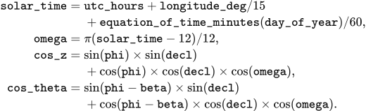
Longitude and the time correction give local solar time and hour angle. longitude_deg is positive eastward, solar_time is in hours and omega is in radians. incidence_cosines converts latitude and tilt to radians as phi and beta, returning cos_z and cos_theta for the zenith and incidence angles:
Diffuse radiation and array-plane irradiance
The horizontal irradiance is decomposed into diffuse and beam components. plane_of_array sets ghi to the non-negative part of ghi_kw_m2, in kW/m², and calculates extraterrestrial_normal as parameters.solar_constant_w_m2 / 1000.0 * eccentricity_factor(day_of_year); the default multiplier is 1.361 kW/m². For positive ghi and zenith below 87°, the clearness index is

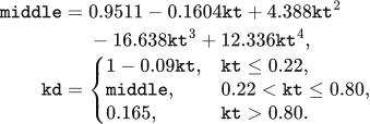
The diffuse fraction follows the hourly relation of Erbs, Klein and Duffie (1982), Solar Energy 28(4), 293–302. The coefficient kd depends on the dimensionless clearness index kt; middle is the polynomial value for its central interval:
The Hay–Davies (1980) transposition combines beam, sky-diffuse and ground-reflected irradiance. dhi, bhi and dni denote diffuse horizontal, beam horizontal and direct normal irradiance in kW/m². anisotropy, beam_ratio, sky_view and ground_view are dimensionless; the default albedo is 0.2. The array-plane irradiance poa is
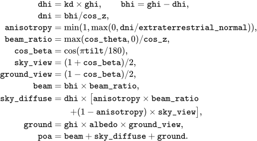
Periods with zenith at or above 87° or with zero ghi have kt=0, kd=1, dhi=ghi, bhi=0, dni=0, anisotropy=0 and beam_ratio=0. Their poa retains the diffuse and ground-reflected terms. The selected max_zenith_deg replaces 87° in this condition when its parameter is changed.
Array-plane irradiance is converted to generation by the performance ratio and a coefficient ceiling of 1. Under the default parameters, site_cf_by_source returns the dimensionless coefficient values as

The coefficient ceiling is applied after the array-plane step. Horizontal conversion applies the performance ratio to hourly[index] directly. The following algorithm covers wind, instantaneous solar and accumulated solar. ds is the opened NetCDF input, binding declares its time convention, periods is the requested number of half-hours, and method contains clock, loss_factors and plane_of_array:
hourly, evidence = hourly_unit_cf(ds, technology, latitude, longitude, binding)
index = hour_index(periods, len(hourly), method.clock, evidence["time_convention"])
values = hourly[index]
poa_applied = False
if technology == "solar" and method.plane_of_array:
    poa_applied, reason = plane_of_array_applies(method, evidence["time_convention"])
    if poa_applied:
        values, poa_evidence = plane_of_array(values, latitude_deg=latitude,
            longitude_deg=longitude, parameters=plane_of_array_parameters())
multiplier = method.multiplier(technology)
values = values * multiplier
if poa_applied:
    values = np.minimum(values, 1.0)
return values
Project locations and weather mixtures
Assets obtain their representative weather from technology and location. The GB template lists 11 solar and 11 onshore points and 21 offshore point names; the R029 2025 stock has 11 solar, 11 onshore and 18 offshore assets with positive capacity. Operating stock is mapped during the initial selection in Chapter 2. Planned projects receive a representative point before commissioning.
A planned project's explicit location takes precedence. attach_project_weather first uses its latitude and longitude, then searches the source REPD row by physical_project_id, then uses the site name when coordinates remain missing. Finite coordinates are assigned to the nearest representative of the same technology. nearest_site converts project coordinates to radians as lat1, lon1 and representative coordinates as lat2, lon2; the distance in kilometres is
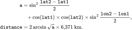
Equal distances select the first representative in the declared order. Solar and onshore planned projects with missing coordinates use their REPD region and the following city mapping. The initial operating-stock reader also uses this table, with the region taking precedence over coordinates at that earlier step.
| REPD region | Representative point |
|---|---|
| East Midlands | Nottingham |
| Eastern | Ipswich |
| London | London |
| North East | Newcastle |
| North West | Manchester |
| Scotland | Edinburgh |
| South East | Portsmouth |
| South West | Bournemouth |
| Wales | Cardiff |
| West Midlands | Birmingham |
| Yorkshire and Humber | Sheffield |
Unlocated projects share a capacity-weighted weather mixture when they enter operation. commissioned_project_weather first accumulates each representative's operating capacity as stock[name] and adds all explicitly located projects due in that year. It then groups the remaining projects by technology. total_stock is the corresponding stock in MW, total_new is the new MW and names is the list of that technology's representatives:
total_stock = sum(stock[name] for name in names)
total_new = sum(p.capacity_mw for p in projects)
if total_new <= 0 or total_stock <= 0:
    weights = {names[0]: 1.0}
else:
    names.sort()
    remaining, weights = total_new, {}
    for i, name in enumerate(names):
        amount = remaining if i == len(names) - 1 else total_new * stock[name] / total_stock
        remaining -= amount
        weights[name] = amount / total_new if amount > 1e-6 else 0.0
Each project in the unlocated group receives the same weights. Positive allocations above 0.000001 MW become amount / total_new; smaller allocations have zero weather weight. Alphabetical ordering and the final-point remainder fix the floating-point allocation order. With zero total stock, the first representative receives weight 1.
The stored weather_source_weights remain attached to the asset after commissioning. source_weights uses this explicit mapping first, then a single weather_source_asset_id, then an identity match through the asset, assigned generator, investment owner, source agent or base asset. Source names must identify representatives of the same technology. Weights must be finite and non-negative, with their sum at most 1 plus 0.000000000001. If deficit = 1.0 - sum(weights.values()) exceeds that tolerance, cohort is the positive finite weather_allocation_cohort_mw and skipped counts zero weights; acceptance requires deficit <= skipped * 1e-6 / cohort + 1e-12.
The asset's availability is the weighted sum of its source curves. _map_lineages applies the mapping weights to each source's values; using subscript name to select the source array, the resulting combined is

Zonal allocation preserves the weather curve while dividing the asset's physical capacity. StagedBidAtCostPSM multiplies capacity_mw by each share; the shares sum to 1. It multiplies storage charge_power_mw, discharge_power_mw, energy_capacity_mwh and initial_soc_mwh by the same share. Chapter 7 defines the asset-to-zone mapping and network constraints.
The optional REPDERA5AggregatedWeather.build interface combines caller-supplied project curves within each owner–technology–zone group. For allocation records rows, total is total MW, values is a project's dimensionless curve and weighted is the group's curve:

This aggregation requires equal-length, finite project curves in [0,1] and positive total. Multiplication of weighted by total MW gives the sum of the projects' available power. The zonal dispatch interface can instead use the representative curve directly for each allocated portion of an asset.
Technology-average investment profiles
Annual expansion calculations use one technology-average profile for solar, onshore wind and offshore wind. These inputs combine 2022 ERA5 data with the fleet and project assumptions embodied in sa.csv, wa.csv and we.csv. Each public2 file contains 8,760 hourly values and declares interval_minutes=60; each value supplies two consecutive half-hours in source row order.
The resulting availability is dimensionless and supplies peak and annual capacity headroom in Chapter 6. These investment profiles enter that rule directly. Dispatch availability follows the site sampling, time assignment, conversion and losses defined above.
4 Operation and storage
VALUE resolves demand and supply in half-hour periods, with generation, imports, exports and storage subject to their physical capacities. This chapter defines the operating clock, staged market clearing and storage-cost calculation. Chapter 5 gives the national Native dispatch algorithm, Chapter 7 adds network constraints, and Chapter 6 links annual operating results to investment.
Operating clock and initial storage
A model year contains 365 days and 17,520 half-hour periods in UTC. period_start_utc takes the zero-based period, divides it into day_index and within-day offset, and adds offset×period_hours hours to the date returned by model_day. With period_hours=0.5, the calculation is:

model_day skips 29 February. Source series are aligned to this clock before dispatch; records declared as Europe/London are converted to UTC row by row. Output timestamps use ISO 8601 with Z. Period energy is measured in MWh, rated power in MW and inventory in MWh.
Storage has a specified opening inventory at each model-year boundary. Native creates each year's storage agents with empty stored_energy; Chapter 5 defines the within-year batch updates. The chronological input used by staged, LP and DC dispatch assigns initial_soc_mwh=0.5×energy_capacity_mwh. These opening conditions apply each year. The preceding year's delivered sales and holding-time observations are retained for storage-cost preparation.
Ahead market and balancing
The staged PSM clears forecast demand before balancing actual demand. For each non-storage resource, _ahead_offers reads the period availability and marginal cost. availability is the supplied availability clipped at zero; physical_cost is the period-specific cost when supplied, otherwise the constant marginal cost. multiplier, from market.bid_multiplier, defaults to 1. The offered energy and price are:

A storage offer is bounded by discharge power and stored energy. soc[resource.asset_id] is opening stored-side inventory, and discharge_efficiency converts it to delivered energy:
available_mwh = min(
    resource.discharge_power_mw * model_input.period_hours,
    soc[resource.asset_id] * resource.discharge_efficiency
)
clear_ahead sorts offers by price_gbp_per_mwh, then offer_id. It begins with remaining=forecast_demand_mwh, accepts the smaller of remaining demand and each offer’s available energy, and reduces remaining demand by that quantity. The last accepted price becomes clearing_price_gbp_per_mwh; all accepted energy receives that price. Clearing stops at a remaining demand of 10⁻¹² MWh. Zero accepted supply has a zero clearing price; the remaining forecast shortfall enters unserved_forecast_mwh.

Balancing responds to the difference between actual demand and the ahead schedule. In CopperplateBalancing.clear, final_dispatch initially equals schedule_mwh_by_asset, and gap_mwh=real_demand_mwh−sum(final_dispatch.values()). Generation and imports offer their unused available energy upward and their scheduled energy downward. Storage can first withdraw scheduled discharge and then charge within its power, energy and efficiency limits. Exports enter as negative injections at the declared connection location and capacity.
Downward bids and settlement
Downward settlement returns the accepted reduction multiplied by its bid price. Thus an upward adjustment has positive signed delta, a downward adjustment has negative delta, and both use cashflow=delta×price_gbp_per_mwh. The staged and network pathways construct these prices with network-economic-v2.
Thermal downward bids divide the ahead schedule into the running range and the minimum-stable-output segment. thermal_dec_segments sets shutdown_mwh=min_stable_fraction×scheduled_mwh and puts the remainder in running_mwh. Running-range price is avoided marginal cost after the downward multiplier and policy support. Shutdown price deducts restart expenditure spread across the expected shutdown interval. In RestartParameters.net_saving, avoided_cost is GBP/MWh, restart_cost(horizon_h) is GBP/MW per start, and horizon_h is hours:

shutdown_horizon_hours counts the current period plus consecutive later periods whose forecast demand is covered by declared VRE and nuclear availability. Its returned duration is (1+run_after[period])×period_hours. When this duration is shorter than min_down_time_h, last_resort_price places the shutdown bid at least 0.01 GBP/MWh below the lowest rounded ordinary downward bid. Otherwise the shutdown price is its net saving. With an empty ordinary-bid set, net saving supplies the price.
CCGT uses a minimum stable fraction of 0.50, minimum downtime of 6 h and hot, warm and cold restart costs of 113.7, 134.4 and 155.0 GBP/MW. OCGT uses 0.50, 0.5 h and 175.7 GBP/MW; biomass uses 0.35, 6 h and 129.2 GBP/MW. CCGT selects hot starts below 12 h, warm starts from 12 through 48 h and cold starts above 48 h. These costs are in 2025 GBP. The running range precedes the unit’s shutdown segment; the shutdown segment precedes unsupported wind only when its net saving is positive. Wind precedes shutdown at a price tie.
Other downward prices use resource_dec_price. Imports return marginal×dec_multiplier; wind, solar and run-of-river hydro return −support; nuclear returns marginal×dec_multiplier−support−premium; other fuel resources return marginal×dec_multiplier−support. market.dec_multiplier defaults to 1 and is at most market.bid_multiplier. Unlisted policy support is zero, while nuclear’s default premium is 100 GBP/MWh. Storage values downward adjustment at its upward bid multiplied by round-trip efficiency. storage_dec_price also applies the lowest available upward price and the store's own upward price as bounds; all prices in this calculation are GBP/MWh:
value = up_price_gbp_per_mwh * charge_efficiency * discharge_efficiency
if lowest_inc_price_gbp_per_mwh is not None:
    value = min(value, lowest_inc_price_gbp_per_mwh)
value = min(value, up_price_gbp_per_mwh)
Copperplate balancing ranks upward bids by increasing price, with storage after generation at a price tie; bids above VoLL remain outside the accepted set. It ranks downward bids by decreasing price rounded to 0.01 GBP/MWh, then by class, then by exact price. The class order is fuel running range, imports, storage, run-of-river hydro, VRE, thermal shutdown, nuclear and short-downtime shutdown. Equal-price bids of the same direction and class share acceptance in proportion to available energy.
For each equal-price group, total is available MWh and fraction is the smaller of the imbalance-to-available ratio and 1. The resulting delta changes final_dispatch and earns cashflow. Positive residual demand becomes blackout_mwh. Final supply plus blackout must match actual demand within 10⁻⁸ MWh. Zonal balancing applies the same schedule and bid definitions inside the Chapter 7 network constraints, with exact-price optimisation followed by physical tie-breaking.
A 50 MWh forecast illustrates the two settlements. Wind offers 30 MWh at £0/MWh and gas offers 30 MWh at £60/MWh. The ahead schedule accepts 30 MWh of wind and 20 MWh of gas, paying £3,000 at the common £60/MWh price. If actual demand is 55 MWh, gas supplies 5 MWh more and receives £300 in balancing. Gas physical expenditure is based on its final 25 MWh and equals £1,500.
Storage inventory and bidding
Storage inventory follows final net injection in each period. In CopperplateBalancing.clear, opening is initial stored-side MWh and dispatch is final MWh delivered to the grid; a negative value denotes charging. The updated soc is:

Inventory remains between zero and energy_capacity_mwh, with a 10⁻⁸ MWh rounding tolerance. Charging and discharging respect charge_power_mw×period_hours and discharge_power_mw×period_hours. Zonal dispatch represents these directions separately and requires at most one to exceed 10⁻⁸ MWh. The closing inventory becomes the next period's opening; the annual opening conditions are specified above.
DynamicAnnualStorageCost divides equipment-cost recovery into cycle depreciation and holding recovery. capital_recovery_factor uses discount_rate and lifetime_years; at a nonpositive discount rate it returns the inverse lifetime, otherwise it uses:

Annual cost is annualised asset CAPEX plus fixed maintenance. prepare_year takes actual asset capital_cost_gbp, power_capacity_mw, energy_capacity_mwh and discharge_efficiency. Catalogue lifetime, duration, cycle life and fixed-maintenance rate come from spec. The calculation keeps the asset’s declared energy-to-power ratio.
capex = max(capital_cost_gbp, 0)
annualized_capital_cost_gbp = capex * capital_recovery_factor(
    discount_rate, spec.economic_lifetime_years)
annual_fixed_opex_gbp = (
    max(power_capacity_mw, 0) * 1000 * spec.fixed_opex_gbp_per_kw_year)
annual_levelized_project_cost_gbp = (
    annualized_capital_cost_gbp + annual_fixed_opex_gbp)
Reference annual sales use the smaller of lifetime cycles per year and physically possible charge-discharge cycles. _reference_observation calculates life_cycles_per_year from cycle life, physical_cycles_per_year from charge-discharge duration, and their minimum cycles_per_year. It then obtains annual delivered sales sold in MWh and holding time dwell_periods in model periods:
life_cycles_per_year = spec.maximum_cycles / spec.economic_lifetime_years
physical_cycles_per_year = 8760 / max(2 * spec.duration_hours, 1e-9)
cycles_per_year = min(life_cycles_per_year, physical_cycles_per_year)
sold = (max(energy_capacity_mwh, 0) * max(discharge_efficiency, 0)
        * cycles_per_year)
dwell_periods = max(spec.duration_hours / period_hours, 2)
The pricing basis uses previous-year sales when positive, subject to a floor tied to reference sales. reference is the observation returned by _reference_observation; it stores sold in sold_energy_mwh and its reference holding time in average_dwell_periods. previous holds the preceding year’s observation. The selected basis_sold is MWh and average_dwell is the delivered-MWh-weighted number of holding periods:
observed = previous
minimum_sold = reference.sold_energy_mwh * max(utilisation_floor, 0)
if observed.sold_energy_mwh > 0:
    basis_sold = max(observed.sold_energy_mwh, minimum_sold)
    average_dwell = max(observed.average_dwell_periods, 2)
else:
    basis_sold = reference.sold_energy_mwh
    average_dwell = reference.average_dwell_periods
Defaults are utilisation_floor=0 and discount_rate=0.05. Batteries recover cycle depreciation from delivered MWh; pumped hydro and hydrogen have a zero cycle-depreciation component.
usable_cycle_output = energy_capacity_mwh * discharge_efficiency
cycle_depreciation_gbp_per_mwh = (
    capex / (usable_cycle_output * spec.maximum_cycles))
expected_cycle_recovery = cycle_depreciation_gbp_per_mwh * basis_sold
remaining_annual_recovery = max(
    annual_levelized_project_cost_gbp - expected_cycle_recovery, 0)
weighted_basis = basis_sold * max(average_dwell, 1)
holding_recovery_gbp_per_mwh_period = (
    remaining_annual_recovery / weighted_basis)
The cycle term is zero when has_cycle_depreciation is false or either denominator factor is zero. The holding-recovery term is zero when weighted_basis=0. Under Native's cycle_only bid setting, bid_price_gbp_per_mwh returns cycle_depreciation_gbp_per_mwh: the three battery types bid their cycle wear, while pumped hydro and hydrogen bid zero. Equal-priced storage batches are released in charging order, oldest first.
The storage-cost calculation also reports recovery per holding period. The linear holding-price calculation is cycle_depreciation_gbp_per_mwh + max(dwell_periods,0)×holding_recovery_gbp_per_mwh_period. Staged dispatch passes dwell_periods=0, so its holding-price contribution is zero. The catalogue provides the life, cycle and maintenance parameters listed in Chapter 2; fixed maintenance is 13.4 GBP/kW/year for pumped hydro, 6.6 for the three battery types and 19.7 for hydrogen.
Sales update the following year's cost basis. record_sale takes delivered MWh and the number of periods since charging, and accumulates sales and sales-weighted holding time in current. Its average_dwell_periods is the weighted total divided by sales when sales are positive, and zero otherwise:
delivered = max(delivered_mwh, 0)
dwell = max(dwell_periods, 0)
current.sold_energy_mwh += delivered
current.dwell_weighted_sold_mwh_periods += delivered * dwell
At year-end, storage_cost_observations records these quantities by storage agent. The next annual preparation takes them as previous, calculates the new recovery amounts and resets current to zero. This observation update supplies the cost calculation while the physical inventory follows the opening conditions and dispatch updates given above.
5 National market clearing
The national market clears forecast demand and then balances actual demand at one node in each half-hour. The default module value-bid-at-cost-psm applies native-corrected-v1: generators and imports offer available power, storage offers eligible energy batches, and the realised dispatch advances the physical state to the next period.
Inputs, agents and availability
Dispatch quantities are powers in MW, with period_hours = 0.5. The variables forecast_demand, real_demand, capacity_limit, real_gen_energy and alter_limit respectively describe forecast demand, actual demand, available output, realised output and the per-period ramp allowance. The generator index is  , the time index is
 , and other asset indices are defined with each calculation. The UTC model year has 17,520 periods. The native kernel reads demand in MW and multiplies accepted power by
period_hours for MWh output and settlement. The canonical_psm_data.py chronology supplies period MWh to staged and optimisation modules, following Chapter 2.
Generator bids combine operating cost with a start-up adder determined by the previous accepted set. Gas and biomass use gen_cost + fuel_cost + carbon_price + unit_time_cost; nuclear, renewables and natural-flow hydro use gen_cost + unit_time_cost. The input-row costs are summed into the runtime agent’s gen_cost, in GBP/MWh; carbon_price is already an expenditure per MWh. For bid multiplier  , composite operating cost
 and start-up adder
 ,

The bid multiplier defaults to 1. Hydro and renewables have zero start-up adders. The GB input rows give biomass a composite cost of 0.2 + 80 + 4.8 = 85 GBP/MWh and a start-up adder of 83 GBP/MWh; CCGT and OCGT composite costs are 55.07 and 74.92 GBP/MWh. Biomass receipts follow market settlement.
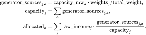
The annual adapter maps operating and newly commissioned assets to market agents first by name, then by technology and normalised region. Multiple matches use previously mapped capacity, constructor capacity, or equal shares in that order. weights and total_weight allocate each asset's capacity_mw into generator_sources; these capacities are MW, with  indexing market agents and
 assets.
_allocate_runtime_income distributes raw_income into the asset account allocated, both in GBP, in proportion to the mapped capacities:
Wind uses a 20 MW reference unit and multiplier  ; solar uses a 1 MW reference unit and multiplier
 . Storage power and energy are aggregated by technology.
scheme_c_native_psm.py creates the year's agents and restores prior sales and sales-weighted holding time for bidding. Each year creates storage agents with empty stored_energy; the preceding year's closing inventory is counted as discarded energy in storage_year_boundary.
Renewable availability uses the same period arrays as the canonical input adapter. site_weather.site_cf_by_source computes the Chapter 3 weather, loss and plane-of-array transformations, and kernel_injection.KernelSiteInputs supplies the resulting capacity factors  to the kernel:

Nuclear availability preserves each station's PRIS reference output when converting to model capacity. nuclear_load_factor reads pris_load_factor, pris_reference_mw and capacity_mw. generation_end_period supplies end, the first period after the announced end month; a station with year-round availability retains its factor throughout the year. With  indexing stations,
asset_availability produces the station array values, and kernel_availability combines it by capacity:
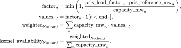
The fixed 2019–2024 mean load factors are 0.668 for Heysham 1, 0.689 for Hartlepool, 0.752 for Heysham 2, 0.792 for Torness and 0.801 for Sizewell B. Station-policy inputs set the four AGR stations' availability to zero from period 4,320 of 2030, 1 April 00:00 UTC. Sizewell B retains full-year coverage until its declared retirement year. Fallback load factors are 0.801 for new PWR/EPR stations, 0.727 for an unspecified AGR and 0.723 for an undifferentiated national nuclear asset. GBP1 public2 applies the VALUE-UK nuclear station policy (value_uk_nuclear_policy_v1.json: five EDF stations and their declared generation ends), while its fleet input table contains one aggregate nuclear row; R029 retains a national aggregate and uses 0.723 under national dispatch. These parameters are supplied by value_uk_firm_availability_v1.json and firm_availability.py.
Natural-flow hydro combines the DUKES 6.3 mean annual load factor with a monthly shape derived from quarterly Energy Trends data:


The shape has an arithmetic monthly mean of 1 and a 365-day weighted mean of 0.99883, giving a model-year availability of 0.3483. Nuclear and hydro use these fixed profiles across model years.
Nuclear begins the year in service and belongs to  ; gas and biomass begin outside that set. The generator parameter rows provide opening
real_gen_energy, and nuclear initially sets it to capacity_limit. Hydro and biomass initialise have_gen_energy to their opening real_gen_energy. Each period adds add_energy to energy_limit, accepts generation against the remaining budget, and returns curtailed generation to that budget. The budget quantities are MW-periods; multiplication by period_hours gives MWh.
Storage offers and period positions
The storage agent records each charging period's stored-side MWh in stored_energy, indexed by the charging period  ;
 denotes the current period.
Battery.charge limits input by power_capacity_mw, energy_capacity_mwh, charging efficiency n_1 and remaining power after the current period's earlier charging. For each battery, the implementation calculates
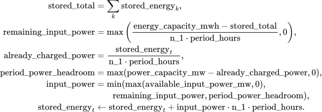
Battery.discharge withdraws output_power * period_hours / n_2 MWh from the selected batch, where n_2 is discharging efficiency. All batches and stages share rated power. Ahead offers use existing batches; upward balancing uses batches aged at least two periods. The period book's discharged_mw and charged_mw, and the sum of stored_energy, satisfy

Surplus absorption first buys back the store's discharge from the same period and returns the withdrawn energy to its original batches. Further surplus can charge the store after its remaining discharge reaches zero. A store that has charged offers zero discharge in later stages. Surplus absorption processes forecast surplus before other available surplus and record sales at the closing net position. Ahead storage remuneration remains payable on bought-back output.
Self-discharge multiplies inventory by  each period. The values of
 are 0.000021 for batteries and other default types, 0.000001 for pumped hydro and 0.000005 for hydrogen storage. Batches below 0.001 MWh are removed and included in inventory reconciliation.
The default dynamic storage-cost module uses cycle depreciation in storage bids. Batteries bid  ; pumped hydro and hydrogen storage bid zero. Oldest batches are offered first:

Chapter 4 defines the storage state and bid-cost calculation. Annual delivered MWh and sales-weighted holding time supply the following year's pricing inputs; Chapter 6 defines their cost treatment.
Forecast clearing and balancing
Market clearing orders generator, import and storage-batch offers by a stable key. Within the same 0.01 £/MWh band, generation and imports precede storage; unrounded price and input order resolve further ties:

An ordinary generator serves residual forecast demand up to

Hydro and biomass also obey their remaining cumulative budget  , expressed in MW-periods and converted to MWh by
 . Nuclear acceptance can exceed residual demand
 : when its upper limit is larger than
 , it supplies
 . This excess becomes already-generated, inflexible surplus. Renewable availability above accepted demand is retained as available surplus.
Interconnectors offer positive available import capacity into the ahead market at the external price multiplied by  . Their offers carry capacity limits with zero ramp and start-up adders. Balancing offers only
 . Negative transfer capacity represents export capability, accepted at positive external prices.
Surplus accounting rebuilds renewable surplus from availability minus accepted output after the ahead stage. Already-generated nuclear surplus is used first. When renewable surplus supplies storage, exports or flexible demand, it enters gross renewable generation. Recorded vre_accepted is therefore gross VRE output, curtailed is available VRE minus gross output, and excess is non-VRE spill. Nuclear surplus already included in ahead supply and settlement serves balancing demand once; renewable surplus entering supply during balancing receives balancing settlement.
Ahead clearing accepts successive offers until residual forecast demand reaches zero or all offers are exhausted. An ahead period with no accepted nuclear generator multiplies nuclear real_gen_energy by 0.99 before balancing. At the end of realisation, each generator with zero final dispatch sets real_gen_energy to zero; dispatched generators carry their final output into the next period.
The real-time branch compares actual and forecast demand. A lower actual value invokes surplus absorption and downward dispatch; a higher or equal value invokes upward balancing. This comparison also applies when ahead supply falls short of the forecast. In that case, the lower-demand branch still requests a reduction of  ; any remaining unmet demand enters the energy account below.
accepted_bids = initial_running_rows(generators)
for period in range(periods):
    Read availability, forecast_demands[period], real_demands[period]
    Read period external_price and transfer_constraint
    ahead_market_bidding(...):
        Add add_energy to each hydro/biomass energy_limit
        Apply storage self-discharge; construct offers
        Sort by merit_key; accept forecast demand subject to physical bounds
        rebuild_surplus(...); uniform_income(...)
    realise_period(...):
        if real_demand < forecast_demand:
            curtailment_market_bidding(...):
                Buy back discharge, charge, export, supply electrolysis
                economic_downward_stack(...): reduce remaining output
        else:
            balancing_market_bidding(...):
                Use surplus; buy back discharge and charge
                Offer eligible batches, generation and residual imports
                Export remaining surplus and supply electrolysis
                Clear upward demand; record remaining blackout
        Set real_gen_energy to zero for generators with zero final output
    battery.close_period(period) for each battery
    physical_cost_terms(...): record period expenditure components
return period dispatch, prices, income, inventory and annual totals
Surplus absorption visits storage in ascending order of storage_fee, per_storage_fee and n_1 * n_2 in the lower-demand branch, and in input order in upward balancing. Within each store it buys back current-period discharge before charging. Positive-price exports follow descending external price in the lower-demand branch and ascending external price in upward balancing, each bounded by the absolute negative transfer_constraint.
Upward clearing starts from the last ahead-accepted generator and includes later generator offers, storage batches at least two periods old, and unused import capacity. For that marginal generator, valid_energy is its current ramp-limited output bound less ahead-accepted MW; later generators use their full ramp-limited bounds. Hydro and biomass also retain their remaining budgets. Each accepted quantity reduces energy_provided, initially real_demand - forecast_demand; clearing ends at zero or after the final offer, and the remaining quantity becomes blackout.
The common electrolyser absorbs surplus as flexible demand. Its source parameters are 10 MW capacity, a 0.125 MW-per-period ramp and conversion efficiency 0.65; the data-pack parameter row supplies the selected values. Available wind and solar enter market clearing first, followed by surplus allocation to storage, exports and electrolysis. The electrolyser limit for this period is energy_cell = min(real_energy + rampup_rate, capacity_limit), in MW. Its accepted min_value is the smaller of this limit and remaining surplus: excess_energy + need_curtailed_energy in the lower-demand branch, or excess_energy in upward balancing. It updates real_energy = min_value and green_hy = min_value * energy_efficiency.
Economic downward order
Downward dispatch compares avoided operating expenditure after storage, exports and flexible demand absorb surplus. ramp_floor_mw returns the larger of zero and previous real_gen_energy less alter_limit; VRE and imports have zero floor. avoided_cost uses the asset's composite gen_cost, subtracting NUCLEAR_DEC_PREMIUM_GBP_PER_MWH = 100 for nuclear; imports use external_price. Ordinary rows follow descending avoided cost rounded to two decimal places.
Gas and biomass split their accepted ahead output  into a running range and a shutdown segment. Here
 represents the aggregate's online capacity for this ordering rule, and
 is the minimum stable fraction:

The running segment avoids  £/MWh. The shutdown segment compares avoided expenditure over expected downtime
 with restart expenditure
 , measured per MW of capacity per start:

SurplusOutlook.run_after counts consecutive periods after the current one with forecast demand no greater than forecast wind, solar and nuclear availability. The current downward period adds one period. Without injected availability arrays, horizon_h = 0.5 h. Removing one MW at the stable fraction shuts 1 / min_stable_fraction MW of capacity; the restart comparison divides restart cost by that fraction and by the expected downtime.
A shutdown segment with  enters the same descending net-saving order as other resources. Positive
 precedes zero-cost VRE; zero or negative
 follows VRE, including ties after rounding. A segment with
 follows all other reducible resources. These quantities define a continuous dispatch-ordering rule; the physical cost account uses the start-up bid adder
 defined above.
| Technology | Restart cost: hot / warm / cold, 2025 GBP/MW | Minimum stable fraction | Minimum downtime, h |
|---|---|---|---|
| CCGT | 113.7 / 134.4 / 155.0 | 0.50 | 6 |
| OCGT | 175.7 / 175.7 / 175.7 | 0.50 | 0.5 |
| Biomass | 129.2 / 129.2 / 129.2 | 0.35 | 6 |
CCGT uses the hot value for  h, warm for
 h, and cold for
 h.
value_thermal_restart_v1.json combines cycling-wear estimates from Kumar et al. (2012) with GB start-up fuel and carbon estimates from Staffell and Green (2016). Its minimum-load and downtime assumptions draw on Elexon declarations and the technical sources recorded with the table. The table converts the selected 2024 GBP values to 2025 GBP using ONS CPI D7BT,  , and rounds restart costs to one decimal place; the recorded conversion factor is 1.0336.
RestartParameters.break_even_hours divides restart cost by min_stable_fraction times avoided operating cost. At the supplied GB costs, break-even times are 4.13 h for hot-start CCGT, 4.69 h for OCGT and 4.34 h for biomass. Thus eligible CCGT and biomass shutdowns at 6 h have positive net savings; OCGT first has positive savings at 5 h on the half-hour grid. The CCGT six-hour cost threshold is 113.7 / (0.5 × 6) = 37.9 £/MWh.
Equal rounded savings use class ranks thermal 0, imports 0.5, hydro and biomass 1, VRE 2, shutdown segments 2.5 and nuclear 3, followed by name and input order. Each accepted reduction consumes the remaining requirement once:

limit is the segment's reducible MW, item[2] is its remaining accepted output, and remaining is the outstanding downward requirement. Hydro and biomass reductions return energy to cumulative budgets. Output held by the ramp floor becomes in-dispatch spill. native_corrected.economic_downward_stack applies these reductions. Reduction stops when remaining is at most  MW or every reducible segment is exhausted.
Settlement, displayed price and physical cost
The market dispatch pays every accepted supply category the same marginal price within each stage. Ahead settlement takes the highest accepted offer including imports and storage. uniform_income multiplies accepted power_mw by period length and the stage's price_gbp_per_mwh; the balancing price also includes accepted import prices. income is GBP, power_mw is MW and the price is GBP/MWh; an empty accepted category contributes zero to the maximum:


Storage charges are settled within the current period. Bought-back storage output retains its ahead-stage remuneration, while the physical dispatch and annual delivered-energy totals use the closing net position.
The displayed market price is labelled “Average period cost (£/MWh demand)”. If  is the accumulator of accepted-offer, storage, downward and upward charges, its unit is GBP/hour. The price in GBP/MWh and associated period expenditure in GBP are

This statistic describes expenditure per MWh of actual demand. Generator and storage income are calculated from the settlement accounts above.  includes the current period's storage fee only. Final boundary supply enters the annual generation statistic, with storage discharge reported separately.
Physical operating expenditure values realised generation at composite gen_cost, imports at external_price, and accepted starts at startup_cost times generated MWh. physical_cost_terms returns generation_variable_gbp, import_variable_gbp and startup_adder_gbp for each period. Chapter 6 combines these components with storage depreciation, shortage valuation and annual capital costs.
Energy balance and annual outputs
The period energy balance includes gross accepted supply, charging, exports, flexible demand and non-VRE spill. All quantities in this section are MWh. With accepted supply  , recorded blackout
 , actual demand
 , storage charge
 , exports
 , flexible demand
 and non-VRE spill
 , the period residual is

The energy account absorbs small floating-point residuals through compatibility_adjustment_mwh. This numerical term is applied only within the period tolerance:

The energy account measures total unmet demand from the physical residual and the dispatch branch's recorded blackout:

A period with unmet demand alone closes at  . Consecutive periods with a shortfall form one event within the year. Annual outputs contain event count, period count and unserved MWh; Chapter 6 uses served demand after subtracting each shortfall component once.
The annual output aggregates generator and import MWh, storage charge and discharge, renewable curtailment, non-renewable spill, exports, flexible demand, period prices, asset income and unserved energy. Period states carry realised generation and storage batches forward; the annual model then applies the account and investment rules in Chapter 6.
Back to contents ↑6 Annual accounting and investment
VALUE updates operating capacity once per model year. Annual dispatch supplies electricity sales, operating costs and renewable surplus; these quantities determine investment and retirement. Accepted additions enter a construction pipeline and become operating assets in their completion year. The annual calculation therefore links the current fleet, market income, construction time and future capacity.
Annual inputs and calculation order
The annual input YearState contains the year, operating assets, planning projects and storage-cost observations. Each asset has capacity_mw in MW, optional energy_capacity_mwh in MWh, technology, region and investment owner. Its economic fields contain total capital total_capex_gbp, annual fixed cost annual_fixed_opex_gbp, annualised capital annualized_capital_cost_gbp, lifetime economic_lifetime_years, required annual return preferred_rate and target payback target_payback_years. Chapter 2 specifies the initial fleet, project list and input values.
Projects enter operation before that year's dispatch. SchemeCPlanningPipelineDefinition.advance_year takes each successful project whose expected_completion_year≤state.year, adds its capacity and economic fields to the fleet, and removes it from the active pipeline. Later projects remain in the pipeline. Hydro projects enter operation when their site and hydrological inputs are complete. Failed projects contribute zero operating capacity.
Dispatch produces market, the annual MarketYearResult. Its period summaries contain actual demand, accepted VRE, storage charge and discharge, blackout energy and prices; its asset accounts contain generated MWh and market income. The annual algorithm then computes technology expansion limits, investment quantities, planning admission and the next state in this order:
advanced = planning.advance_year(run, state)
model_input = psm_input_factory(run, advanced.operating_state)
market = psm.run(model_input)
headroom = []
for slot in sorted(expansion_policies):
    policy = expansion_policies[slot]
    headroom.append(policy.evaluate(run, advanced.operating_state, market))
investment_market = adapt_market_for_investment(
    market, advanced.operating_state)
decision = investment.decide(
    run, advanced.operating_state, investment_market, tuple(headroom))
decision = inherit_frozen_zone_shares(decision, advanced.operating_state)
admission = planning.admit_projects(
    run, advanced.operating_state, decision.proposals)
Here advanced.operating_state is the fleet available for the year, headroom contains permitted additions in MW by technology, decision contains new proposals and asset retirements, and admission.next_pipeline contains continuing and newly admitted projects. The input factory applies Chapters 2–3 to the updated fleet; Chapters 4–5 and 7–8 define the selected dispatch calculation. The final state update is given below.
Asset capital and annual system cost
Asset capital is annualised over its economic lifetime with a capital-recovery factor. build_asset_economic_extensions reads total_capex in GBP, life in years and discount_rate, then sets annualized_capital_cost_gbp=total_capex×crf. The factor crf=capital_recovery_factor(discount_rate,life) uses the equation in Chapter 4; the default rate is 0.05. Generation capital is capacity times GBP/MW. Storage capital and fixed maintenance follow the technology catalogue and its declared power or energy basis in Chapter 2.
Annual system cost sums the resource costs of operating assets. The dispatch result supplies total_levelized_capital_cost_gbp, containing annualised capital and fixed maintenance, and total_operational_cost_gbp, containing physical operation. For Native, physical operation comprises the generation and import cost terms in Chapter 5, recorded blackout energy valued at market.voll_gbp_per_mwh (default 17,000 GBP/MWh), and storage cycle depreciation. The restart cost used to rank a downward bid enters that bid's price calculation. Network asset capital and fixed maintenance enter the annual resource account when network expansion is selected.
The system-cost account treats wind, solar and storage fixed maintenance as included in their levelised capital. Their separately recorded maintenance amounts are retained as memorandum items. Existing run-of-river capital recorded under existing_stock_compatibility_capital_gbp is also a memorandum item. Thermal fixed maintenance and commissioned network resource costs enter the cost total.
build_cem_cost_ledger reads the supplied capital total as capital and subtracts the two memorandum amounts as excluded. network_capex and network_fom are annual network capital and maintenance; operating_sum is the sum of the named physical operating components. All costs below are GBP per model year. demand, blackout and served are annual MWh:
network_resource_cost = network_capex + network_fom
non_network_capital = max(capital - network_resource_cost, 0)
excluded = vre_storage_fom + compatibility
headline_fleet_capital = max(non_network_capital - excluded, 0)
headline_capital = capital - (non_network_capital - headline_fleet_capital)
system_cost = headline_capital + operating_sum
served = max(demand - blackout - a2_hidden_unserved_mwh(market), 0)
The variables vre_storage_fom and compatibility hold the wind/solar/storage maintenance memorandum and the existing run-of-river capital memorandum respectively. a2_hidden_unserved_mwh reads additional unserved energy from the annual energy-balance account; it is zero when that account records zero additional shortfall. The output cem_system_cost_gbp=system_cost, and cem_system_cost_gbp_per_mwh_served=system_cost/served for positive served demand. At zero served demand, cost per MWh is left empty. Market payments, policy transfers, construction commitments and residual values have separate accounts; the operating-resource sum uses the physical expenditure terms above.
Annual income and investment groups
Investment groups combine positive-capacity assets with the same owner, technology and region. Owner identity comes from investment_owner_id, then source_agent_id, then the existing asset's identifier. An asset marked investment_eligible=False remains in dispatch and contributes zero endogenous investment. SchemeCAgentInvestmentDefinition.decide processes groups in sorted (owner,technology,region) order.
The investment calculation uses the annual market income attributable to each asset. Native distributes an agent's income over its mapped assets as specified in Chapter 5. For an owner-level settlement, adapt_market_for_investment allocates the owner's income in proportion to operating MW: allocated[asset.asset_id]=income×asset.capacity_mw/capacity, where capacity is that owner's summed MW. Direct asset-level accounts enter the investment calculation as supplied.
Thermal investment income deducts generated electricity times generation, fuel, carbon and unit-time cost. The asset's agent_cashflow row supplies generated_mwh and the four costs in GBP/MWh. Their product gives operating_cost_gbp; operational is the sum over the group's assets. Wind, solar and the three battery types and hydrogen use operational=0. Thus storage investment uses booked ahead and balancing income, including ahead remuneration retained during buy-back. Surplus charging has zero purchase cost, and cycle depreciation and fixed maintenance enter their respective resource-cost accounts above.
For each group, capacity sums operating MW, income sums annual GBP income and replacement sums total_capex_gbp. Unit capital cost cost_per_mw is GBP/MW, roi is annual net income divided by capital, and payback is years:
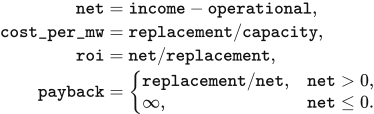
Zero replacement capital gives roi=0. Thermal net is set to zero when abs(net)≤10⁻⁹×max(abs(income),operational), absorbing the difference between sums of the same cashflows. preferred is the largest member preferred_rate, life is the shortest member economic_lifetime_years, and target_payback is the shortest member target_payback_years. Missing or zero values use 0.08, 25 years and life respectively. The initial default asset construction sets biomass, CCGT and OCGT target payback to 25 years. Other initial values are given in Chapter 2. The decision compares the annual input amounts directly through roi and payback.
Annual wind and solar expansion limits
Wind and solar expansion is bounded by peak demand and the technology's available-output profile. In canonical_psm_data, demand is the half-hour energy demand in MWh, period_hours=0.5, availability is the dimensionless technology profile, and capacity_by_technology[technology] is its operating MW. The input uses the investment profiles prepared in Chapter 3. The maximum profile value is peak, and additional capacity headroom is:
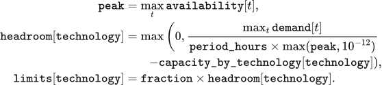
SchemeCVREExpansionPolicyDefinition.evaluate reads fraction from expansion.vre_cap_fraction, default 0.20, and returns limits in MW. For a 1,000 MW peak demand, peak=0.8 and 300 MW operating capacity, headroom=950 MW and the annual limit is 190 MW. A zero profile peak uses the denominator floor 10⁻¹². These limits are calculated separately for solar, onshore wind and offshore wind.
Annual storage expansion limits
Storage expansion uses the renewable surplus remaining after the operating stores have charged. corrected_storage_headroom reads leftover_excess_mwh from storage_headroom_inputs into leftover, and each period's vre_accepted_mwh, real_demand_mwh and storage_discharge_mwh into vre, demand and discharge. These arrays are MWh per period. Surplus available to an additional store and the remaining demand gap are:

A virtual store converts these series into charging and discharging profiles. _simulate_virtual_pool begins with soc=0, has power_mw=10⁹ MW and energy_cap_mwh=10⁹ MWh, and places the round-trip efficiency rte=0.98 entirely on charging. PERIOD_HOURS=0.5; exc, dfc, ch and dis are period MWh. Charging precedes discharging in each period:
max_period_mwh = power_mw * PERIOD_HOURS
soc = 0
charge = zeros(len(excess))
discharge = zeros(len(excess))
for t in range(len(excess)):
    exc = excess[t]
    dfc = deficit[t]
    if exc > 1e-9 and soc < energy_cap_mwh - 1e-9:
        ch = min(exc, max_period_mwh, (energy_cap_mwh - soc) / max(rte, 1e-9))
        soc += ch * rte
        charge[t] = ch
    if dfc > 1e-9 and soc > 1e-9:
        dis = min(dfc, max_period_mwh, soc)
        soc -= dis
        discharge[t] = dis
Charging and discharging energy divided by 0.5 h give charge_mw and discharge_mw. aligned_max_mw finds the largest power exceeded for at least min_hours in both profiles. hours_above_power(power_mw,p_mw) counts values strictly above p_mw and multiplies by 0.5 h. The upper search bound peak is the smaller charging/discharging peak. Zero peak or insufficient hours above zero gives a zero result; min_hours≤0 gives peak. For positive attainable duration, the search starts at lo=0, hi=peak and performs 64 bisection steps:
for _ in range(64):
    mid = 0.5 * (lo + hi)
    if (hours_above_power(charge_mw, mid) >= min_hours
            and hours_above_power(discharge_mw, mid) >= min_hours):
        lo = mid
    else:
        hi = mid
return lo
aligned_utilisation_spectrum applies the search at 730, 365, 52 and 0 hours, producing mw_730, mw_365, mw_52 and mw_0. The successive capacity bands, all in MW, are:
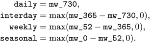
The output stores daily under daily_loop and interday under intraday. corrected_storage_headroom reads the latter into intraday, calculates power_room=max(daily+intraday,0), and sets power_cap=fraction×power_room. Each of 1c_battery, 0.5c_battery and 0.25c_battery receives this separate technology limit. Hydrogen receives hydrogen_cap=fraction×max(seasonal,0). Here fraction comes from expansion.storage_cap_fraction, default 0.20; the weekly band remains a reported quantity. The same year's groups consume their technology's remaining limit in the order defined above.
The storage calculation takes a complete 17,520-period year and its post-charge surplus series. Native dispatch supplies this series. The returned storage limits are zero for a shorter chronology, a period length other than 0.5 h, or an absent post-charge series. This zero rule also defines the storage-investment result when staged, LP or DC dispatch supplies the annual operating result without that series.
Investment quantities and retirement
Each technology follows the eligibility mode in investment_eligibility.json. Solar, onshore wind, offshore wind, the three battery types and hydrogen use headroom_required. CCGT, OCGT, gas and bio_and_waste use explicit_uncapped. Nuclear capacity follows the external project and retirement schedule. Pumped hydro and run-of-river hydro follow site-based projects; the generic profit rule supplies zero proposals for these technologies.
Concurrent expansion rules combine through the smallest limit for each technology. caps holds that minimum, and each year starts with remaining_caps=dict(caps). Earlier projects remain in the construction pipeline; only additions proposed in the current year's investment pass reduce remaining_caps. Several decision years can consequently retain pending projects against the same capacity opportunity.
A group with net<0 and positive cost_per_mw retires capacity. Its retirement is limited by the group's existing MW and allocated to members in proportion to their MW. For other groups, roi>preferred selects Invest_High; otherwise payback≤target_payback selects Invest_Profit; the remaining groups receive Do_Nothing. Both investment classes request net/cost_per_mw. The requested retirement and permitted positive addition are:

For headroom_required, allowed=remaining_caps.get(technology,0) and a positive addition reduces that remaining limit. For explicit_uncapped, allowed=requested. Do_Nothing, nonpositive unit capital cost and nonpositive addition produce zero new capacity. As a numerical example, a 100 MW group with £100 million total capital, £10 million net income, preferred=0.08 and 20 MW remaining headroom has roi=0.10, payback=10 years and requested=10 MW; the resulting proposal is 10 MW before planning success is applied.
New storage retains the group's energy-to-power ratio. For members with energy capacity, duration=sum(asset.energy_capacity_mwh)/capacity hours and proposal_energy=addition×duration MWh. The proposal's economic fields are constructed from technology capital parameters and life; non-storage fixed maintenance is allocated as fixed_om×addition/capacity. Storage capital and maintenance use the catalogue. The proposal retains its investment owner, so its later dispatch income joins that owner's group. In zonal runs, inherit_frozen_zone_shares assigns the new proposal the members' capacity-weighted zone shares.
Construction timing and planning success
Each endogenous addition enters planning at the Application Submitted stage. Initial loading copies development_stage_timelines, repd_status_to_timeline, success_rates and timeline_statistic into state.extensions["planning_parameters"]; subsequent years use the same tables. endogenous_planning_terms reads these tables with the proposal's technology, owner and decision_year.
Technology determines the planning-table labels. Solar uses Solar Photovoltaics, onshore wind uses Wind Onshore, offshore wind uses Wind Offshore, and ordinary batteries and electrolysers use Battery. Gas, CCGT, OCGT and biomass use Wind Onshore. hydrogen_battery uses Solar Photovoltaics. The corresponding timeline keys are solar, onshore, offshore and battery.
The stage table supplies development duration months. _timeline_months normally reads total median duration for Application Submitted; planning.timeline_statistic=mean selects the corresponding mean. A missing technology timeline uses the solar entry, and an absent total mean uses total median. Required durations are finite and nonnegative. The data and initial-project timing rules are specified in Chapter 2.
The duration includes an owner-specific displacement from −6 to +6 months. model_project_key(owner) returns Model Decision: <owner>, and stable_int_hash converts its MD5 result to an integer using the first 16 hexadecimal digits. The following implemented arithmetic gives the completed year. round uses ties to even, so 58.5 months rounds to 58:
key = model_project_key(owner)
jitter = (stable_int_hash(key) % 13) - 6
rounded_months = int(round(max(1, months + jitter)))
year = int(decision_year)
source_completion = year + rounded_months // 12
completion = max(source_completion, year + 1)
The proposal stores completion as expected_completion_year. Thus the earliest endogenous commissioning is the year after the investment decision. For the public2 tables, 2025 offshore proposals complete in 2033 or 2034, onshore in 2029–2030, solar in 2026–2027, ordinary batteries in 2027, and thermal plant in 2030. The VALUE 101 tables use shorter durations, giving 2026 commissioning for 2025 proposals.
Success probability is read by technology label and region. source_success_region maps the solar and onshore owner names' cities to regions: Nottingham–East Midlands, Ipswich–Eastern, London–London, Newcastle–North East, Manchester–North West, Edinburgh–Scotland, Portsmouth–South East, Bournemouth–South West, Cardiff–Wales, Birmingham–West Midlands and Sheffield–Yorkshire and Humber. An owner name containing offshore maps to All Offshore; other owners map to England. _success_rate first takes the matching region, then the arithmetic mean across that technology's regional entries, then 0.75. Probabilities lie in [0,1].
The public2 offshore probability is approximately 0.917; onshore regional values are approximately 0.22–0.71 and solar values 0.84–0.95. Ordinary battery owners use approximately 0.873 and thermal owners approximately 0.547 through the technology-mean fallback. VALUE 101 uses success probability 1. These probabilities apply when the new proposal is admitted into planning.
The default planning.success_mode=expected selects mode=expected_capacity and admits capacity=proposal.capacity_mw×probability. Energy capacity, total capital, annualised capital and annual fixed cost receive the same factor once; unit prices, lifetime and return parameters retain their values. A zero probability gives zero admission. Subsequent years commission the admitted capacity at its scheduled time.
planning.success_mode=stochastic selects mode=seeded_stochastic and admits the full proposal when a deterministic draw is below its probability. seed comes from planning.random_seed, default 0. The proposal identifier combines run.run_id, the decision year, owner and the zero-based index of the sorted investment group. The same input fields yield the same draw; changing the run identifier changes it:
proposal_id = f"{run.run_id}:{market.year}:{owner}:{index}"
digest = hashlib.sha256(f"{seed}:{proposal_id}".encode("utf-8")).hexdigest()
draw = int(digest[:13], 16) / float(16 ** 13 - 1)
success = probability > 0 and (probability == 1 or draw < probability)
capacity = proposal.capacity_mw if success else 0
SchemeCPlanningPipelineDefinition.admit_projects appends admitted projects to the active pipeline. At the start of a later year, a due project becomes an asset named commissioned:<project_id>, carrying its admitted MW, MWh, owner and economic fields. Run-of-river projects require hydrology_profile_id, capital_cost_scope=new_build and new_build_cost_source_id; pumped hydro additionally requires site_constraint_id and energy_capacity_mwh. A due project with missing site fields remains deferred in the pipeline.
State update and annual outputs
Retirements change the following year's capacity and economic quantities. SchemeCStateTransitionDefinition.apply sets next_year=current_state.year+1. If an asset's declared model_unavailable_from_year has been reached, the full asset retires; otherwise the requested retirement applies. resize_asset_economics limits capacity at zero and scales energy capacity, fixed maintenance and capital with the surviving asset:
new_capacity = max(capacity_mw, 0)
ratio = new_capacity / old_capacity
new_energy = old_energy * ratio
total_capex = (capital_cost_per_mw * new_capacity
               + capital_cost_per_mwh * new_energy)
annual_fixed_opex_gbp *= ratio
annualized_capital_cost_gbp = total_capex * capital_recovery_factor(
    capital_discount_rate, economic_lifetime_years)
Here capacity_mw is old capacity less requested retirement, old_capacity and new_capacity are MW, and old_energy and new_energy are MWh for storage. For a project-level capital amount with both unit capital fields equal to zero, total_capex is its previous capital multiplied by ratio. A zero remaining capacity sets the asset status to retired. Economic lifetime determines annualisation and the investment payback fallback; scheduled retirement uses the declared unavailable year or the loss-based retirement quantity above.
The next YearState contains surviving assets, admission.next_pipeline and the year's storage-cost observations. transition_state supplies the commissioned operating fleet, continuing projects and updated observations to transition.apply; its output year advances by one. Physical storage restarts from the Chapter 4 opening conditions, while sales observations feed the next annual cost calculation.
Annual outputs contain dispatch energy, income, system cost, technology limits, investment proposals, planning admissions and next-year capacity. Cost per served MWh uses the account above. Chapter 9 defines operational and embodied emissions, storage-carbon tracing and the construction emissions of optional network additions. At the study horizon, report_only returns the final state, pipeline_tail advances projects already in the pipeline, and full_extension continues annual operation and investment.
7 Transmission and network constraints
Spatial representation of zonal redispatch
Zonal redispatch determines generation adjustments, storage operation and transfers that serve each zone after a national ahead market. Each half-hour uses a lossless transport model: final injections satisfy zonal demand, corridor limits and geographical boundary capacities. The British input contains 23 zones and 22 computational corridors. The DC and AC formulations below use bus and branch inputs.
The British network inputs are supplied in value-uk-research-suite-v1-public2. The zones table defines the regions, corridors gives directed connections, cutsets assigns corridors to geographical boundaries, ratings supplies time-dependent limits, asset-map assigns resources to zones, demand supplies zonal MWh, and interconnector-landings assigns import/export assets to landing zones. B6 and B7a have symmetric capacities of 6,700 and 9,400 MW. The supplied 2025–2034 configuration holds these capacities fixed.
Asset location follows a fixed precedence. _zone_shares_with_source first uses frozen_zone_shares, then matches asset_id in asset-map, then matches it in interconnector-landings, and finally assigns the asset to the single zone marked is_unconstrained_fallback. Shares sum to 1 within a tolerance of  . An asset occupying several zones becomes a physical unit in each zone with capacity, storage power, energy and opening inventory multiplied by its share; all units retain their original investment owner.
The supplied mapping places wind and solar by site and assigns CCGT, OCGT, biomass, run-of-river hydro, nuclear, storage and imports to ENGLAND_FALLBACK. The fallback node connects to the declared central transport zone. Nuclear stations created from the station policy enter through that fallback, including Torness, whose geographical location is north of B6. Import resource names use import:<country>, while landing-table names use interconnector:<line>; exact identifier matching therefore sends these imports to the fallback node. These assignments determine the injections subject to the B6 and B7a constraints.
Demand follows the spatial rule selected for the case. align_zonal_demand preserves the network pack's zonal shares for the 23-zone study and scales them to national scenario demand. Its arrays aligned, output_real, network_demand_mwh_by_zone and network_national_mwh are MWh; zone and period indices are  :

The last zone receives national demand less the sum allocated to the preceding zones. When both national totals are zero, the scale is 1; a positive scenario demand requires a positive network total. The resulting demand_mwh_by_zone enters the period problem with asset locations, realised availability and interconnector import/export envelopes.
Ahead schedule and adjustment bids
The network module builds its ahead schedule from period resource availability and opening storage inventory. _ahead_offers gives each resource capacity_mw * availability * period_hours MWh at its period marginal cost multiplied by market.bid_multiplier, default 1. Storage offers the smaller of its discharge-power limit over the period and soc * discharge_efficiency, at bid_price_gbp_per_mwh(0.0) multiplied by the same factor. clear_ahead orders by price_gbp_per_mwh and then offer_id, accepts the smaller of available and remaining forecast MWh, and stops when the remaining requirement is at most 1e-12 MWh or all offers are exhausted. The last accepted price settles the ahead schedule.
Resource adjustment volumes are measured relative to schedule_mwh_by_asset. _flexibility_bids offers upward MWh equal to the positive part of available MWh less scheduled MWh and downward MWh up to the scheduled quantity. Upward prices use marginal cost times market.bid_multiplier. The network-economic-v2 downward rules use market.dec_multiplier, default 1, and the per-technology support and nuclear-premium inputs:
| Resource | Downward price, GBP/MWh |
|---|---|
| Fuel generation | Marginal cost × downward multiplier − policy support |
| Imports | Period import price × downward multiplier |
| Wind, solar and run-of-river hydro | − policy support |
| Nuclear | Marginal cost × downward multiplier − policy support − inflexibility premium |
resource_dec_price reads policy support from market.policy_support_gbp_per_mwh_by_technology, default zero, and the premium from network.inflexible_dec_premium_gbp_per_mwh_by_technology, default 100 GBP/MWh for nuclear. Gas and biomass split scheduled MWh into running_mwh and shutdown_mwh: the latter equals scheduled MWh times min_stable_fraction. thermal_dec_segments retains the running price and gives the shutdown segment the net_saving calculation and restart table in Chapter 5. The downtime forecast includes the current period and consecutive subsequent periods whose forecast demand is covered by declared wind, solar and nuclear availability, each lasting period_hours. A shutdown shorter than min_down_time_h receives the smaller of its net saving and a price 0.01 GBP/MWh below every other downward price band.
Storage adjustment bids cover the change from scheduled discharge to final discharge or charging. maximum_discharge is the smaller of discharge_power_mw * period_hours and soc * discharge_efficiency; upward volume is max(maximum_discharge - scheduled, 0). Downward volume is scheduled MWh plus the smaller of charging power over the period and remaining internal capacity divided by charging efficiency. storage_dec_price takes the minimum of the storage upward price, that price times round-trip efficiency, and the lowest available upward price in the period when such a bid exists. A declared export envelope adds a downward withdrawal bid at the nonnegative part of its export price.
Storage starts at initial_soc_mwh; each solved final inventory becomes the next period's opening inventory. Generation follows the period availability and accepted adjustment bounds below. The algorithm processes the supplied chronology once in time order, returning final injections, charge, discharge, inventory, corridor flows, unmet demand and settlement for every period.
Adjustment objectives and operating constraints
Redispatch solves four linear objectives in sequence: bid expenditure including shortage cost, adjustment volume, weighted physical throughput and stable variable order. SinglePeriodProblem stores their coefficient arrays as primary_objective, secondary_objective, physical_tie_objective and stable_tie_objective. Each objective is its array's dot product with values, the period decision vector returned by solve_lexicographic.
The decision vector uses the implementation's variable labels. bid:<bid_id> is accepted nonnegative bid MWh; flow:<corridor_id> is signed corridor MWh; load-shedding:<zone_id> is unmet demand; storage-charge:<asset_id> and storage-discharge:<asset_id> are grid-side storage MWh; absolute-flow:<corridor_id> bounds the absolute corridor flow. In the equations, array subscripts carry these existing identifiers.
The primary objective uses the sign of each bid direction. An upward bid contributes its price_gbp_per_mwh times accepted MWh; a downward bid contributes the negative of that payment. Shortage is valued at voll_gbp_per_mwh, default 17,000 GBP/MWh:
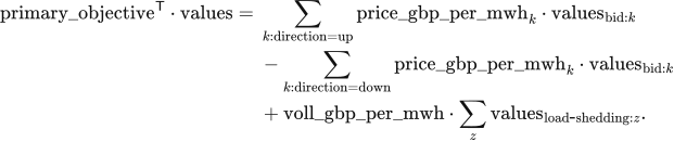
The second objective sums accepted bid MWh and shortage MWh. The third assigns weight 1 to storage charge, storage discharge and absolute corridor flow, plus the class weight of each non-storage downward bid. physical_dec_weight supplies the weights below; bid_dec_rank selects the class:
| Downward class | Weight |
|---|---|
| Fuel plant running range | 0 |
| Import | 0.5 |
| Run-of-river hydro | 2 |
| Wind and solar | 3 |
| Fuel shutdown | 3.5 |
| Nuclear | 4 |
| Fuel shutdown before its minimum downtime | 5 |
Within a zone and at an exact primary-price tie, storage charging precedes run-of-river, wind, solar and nuclear reductions; fuel shutdown follows wind and solar and precedes nuclear. Across zones, class weights also trade against corridor-flow MWh. The primary LP uses exact prices. The fourth objective weights successive variables by 1, 2, … in the fixed order of bid, corridor, zone and storage identifiers.
Final asset injection adds signed accepted bids to the ahead schedule. final_dispatch_mwh_by_asset and schedule_mwh_by_asset are MWh. The index  identifies a bid; its
asset_id selects asset  , and
asset_zone_id_by_asset selects the zone  :
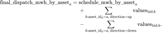
Zonal conservation equates final supply and incoming transfer to demand and outgoing transfer. Corridor direction follows its declared from_zone_id and to_zone_id:

Bid capacity bounds accepted MWh between zero and bid_capacity; MW bids are multiplied by period_hours = 0.5. Shortage lies between zero and zonal demand. Generator injection lies between zero and realised_availability_mw_by_asset times period hours. Interconnector injection lies between negative export_capacity_mwh and positive import_capacity_mwh.
Equal-price non-storage bids share free acceptance proportionally. Upward groups share zone, direction, network effect and price; downward groups also share downward class. _forced_down_by_bid first sets aside the reduction required by actual availability or the interconnector envelope. For a bid and the first bid in its group, the implementation uses

Each geographical boundary limits signed flow across its member corridors. coefficient is the member's direction coefficient; forward_capacity and reverse_capacity are period MWh after converting any MW input:

All boundary constraints apply together. A corridor-specific limit additionally bounds its own flow; absolute-flow is at least both positive and negative signed flow. Thus 6,700 MW at B6 becomes 3,350 MWh per half-hour. Corridors without individual limits remain constrained by zonal conservation and their boundary memberships.
Storage redispatch determines final internal inventory from realised charge and discharge. opening is initial_soc_mwh_by_asset; capacity is energy_capacity_mwh. For each store,

Charging and discharging lie between zero and their respective power limits times period_hours; final inventory lies between zero and capacity. Storage bids use convex_net_power_v1, with at most one bid per direction and a downward price at most the upward price plus  GBP/MWh. Final simultaneous charging and discharging must be at most
 MWh. Final inventory becomes the next period's opening inventory; the national schedule and submitted bids provide the current intertemporal valuation.
Physical resource expenditure is calculated separately from bid payments. resource_cost_gbp_per_mwh_by_asset multiplies positive final injection, and shortage incurs VoLL:

Network constraint cost compares this result with the same LP collapsed to one node, removing corridors and boundaries. solve_network_free_counterfactual retains bids, export arbitrage, import/export envelopes, storage physics, shortage valuation and solver settings. Both cases use the same period unit-cost table: supplied time-varying resource cost, otherwise annual marginal cost, storage cycle depreciation and zero export resource cost. Negative import prices can give negative period resource expenditure.
The primary-objective difference is returned as network_constraint_bid_objective_gbp. It measures the change in accepted bid payments and shortage valuation; physical_resource_cost_gbp measures resource expenditure.
Numerical solution and boundary marginal values
The solver locks total shortage from the primary optimum before bounding its bid-cost component. lock_primary_shedding sets every shortage variable to zero when the primary total is zero; otherwise their sum is bounded above by that primary total. bid_cost_coefficients supplies the bid-only objective for the next bound.
Objective locks use a scale-aware floating-point tolerance. compute_lock_tolerance reads the objective coefficients, the preceding optimum, a unit_floor and the effective solver_tolerance. It computes
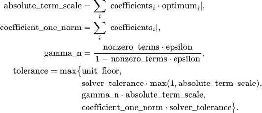
Here nonzero_terms counts nonzero coefficients and epsilon is machine precision. The effective tolerance takes the larger of the applicable solver and bound-canonicalisation tolerances. The bid-cost lock uses a  GBP floor and default solver tolerance
 ; MWh locks use a
 MWh floor and solver floor
 . The bid-cost acceptance ceiling is 1 GBP per period. Each later solve retains the preceding objective bounds. HiGHS dual simplex with presolve uses primal and dual tolerances of
 ; final equality, inequality and bound violations must be at most
 .
for period in the half-hour chronology:
    align_zonal_demand(...): obtain zonal demand
    build_single_period_problem(...): build bids and physical constraints
    solve_lexicographic(problem):
        minimise primary_objective; retain primary boundary marginals
        lock_primary_shedding(...); bound bid_cost_coefficients(problem)
        minimise secondary_objective; retain its objective bound
        minimise physical_tie_objective; retain its objective bound
        minimise stable_tie_objective; validate_solution(...)
    solve_network_free_counterfactual(...): compute matched comparison
    record actual injections, storage inventory, flows, shortage and costs
    pass final_soc_mwh_by_asset to the next period
return all period results
Boundary marginal values measure the primary objective's response to transfer capacity. boundary_marginal_values reads the forward and reverse constraint-row duals before objective locks are added:

A positive boundary value corresponds to a binding forward limit and a negative value to a binding reverse limit. Where binding boundaries share a corridor, several dual allocations can represent the same optimum. The annual output also sums absolute boundary value multiplied by transferred MWh as a congestion measure.
DC network dispatch
The DC network module jointly selects generation, storage operation and nodal voltage angles over the complete chronology. ReferenceDCNetworkPSM builds the variable blocks generation, charge, discharge, soc, blackout, angle and flow in layout. Their solved values carry those names in the equations: the first five are MWh, angle is radians and flow is MW. Resource, storage, bus, branch and period indices are  .
marginal_costs, variable_degradation_gbp_per_mwh_discharged and voll_gbp_per_mwh are GBP/MWh. With fixed assets, operating expenditure is
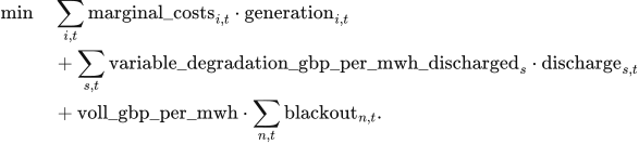
Assets mapped to several buses become independent location-specific units through expand_share_mappings. The mapping field share sums to 1 for each asset and scales its generation capacity, storage charge and discharge power, energy capacity and initial inventory. The solver dispatches these units at their assigned buses and aggregates their outputs by original asset. VoLL reads market.voll_gbp_per_mwh, default 17,000 GBP/MWh.
Nodal conservation converts branch power to energy using period_hours. For units located at bus  ,

Resource bounds multiply capacity_mw, share, availability and period_hours. Storage obeys the charging, discharging and inventory constraints in Chapter 8 with the same mapping share; its transition is

The terminal rule is free, cyclic at initial inventory, or fixed at a declared target. allow_blackout bounds shortage between zero and bus demand when enabled and fixes it at zero otherwise. Availability lies in  , and marginal resource costs are nonnegative.
AC lines and transformers use the declared equivalent reactance and angle difference. base_mva defaults to 100 MVA, tap to 1, and phase converts phase_shift_degrees to radians:

Circuit count scales thermal capacity; the declared equivalent reactance sets the angle equation. Each connected island has one reference bus at zero angle, with other angles bounded by  . Out-of-service branches have zero flow. DC links enter nodal balance as controllable flows within their declared bounds.
HiGHS solves all periods in one linear programme with primal and dual tolerances of  . Completion requires an optimal solver status and an equality-residual limit of
 . Nodal energy-balance duals provide marginal operating prices in GBP/MWh; the displayed system price is demand weighted. The output contains period dispatch, storage inventory, nodal prices and branch flows for the complete horizon.
AC feasibility calculation
The AC module calculates steady-state power flow for a given active-power schedule. Inputs contain active and reactive demand, generator active and reactive limits, voltage setpoints, branch impedances and charging susceptance, fixed taps and phase shifts, voltage bounds and MVA ratings. Each connected island has one slack balancing asset; PV and slack buses require generation, with a common voltage setpoint for generators at one bus. Storage follows its supplied active charging and discharging schedule. PQ buses solve for voltage magnitude and angle from specified active and reactive injections; PV buses hold voltage magnitude and active power; each slack bus holds its voltage magnitude and zero angle while balancing the island.
Nodal complex injection follows the solved voltage and nodal admittance matrix. vm is per-unit voltage magnitude, theta is radians, voltage is complex per-unit voltage, and injection contains MW and Mvar. ybus is per-unit admittance on the base_mva base, and  :

Each branch uses a π impedance representation. _ybus computes series as the reciprocal of resistance_pu plus  times
reactance_pu; charging is half the imaginary charging susceptance; and tap is the tap ratio multiplied by the complex phase-shift factor. The terminal admittances are
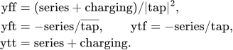
The solver fits active balance at non-slack buses and reactive balance at PQ buses, holding PV and slack voltage magnitudes fixed. The slack asset supplies residual active power and network losses. Nodal reactive generation is checked against the sum of generator limits at that bus. Complex powers s_from and s_to contain MW and Mvar; losses is MW. They use the declared endpoints  :

Apparent power at both terminals is limited by apparent_power_rating_mva times circuits. Every in-service branch enters the admittance matrix with its declared impedance. Topology and device settings remain fixed.
The AC solve starts from flat voltage and from an alternative state with angles spread from 0.01 to 0.03 radians and PQ voltages at the midpoint of their bounds; a declared initial voltage adds a third start. Each start is clipped to the angle and voltage bounds. least_squares uses xtol = ftol = gtol = 1e-12 and max_nfev = 2000. A solution requires successful termination and maximum mismatch at most residual_tolerance, default  MW or Mvar; the acceptable start with the smallest residual is selected.
Accepted AC solutions have start-to-start voltage/angle differences at most  and Jacobian condition number at most
 . Active and reactive generation, voltage and terminal apparent power remain within declared limits to
equipment_tolerance, default  in their respective units. Each period returns voltages, generation, terminal flows and losses. Solving continues through the chronology; an unsuccessful period terminates the calculation.
Optional line expansion
Line expansion screens externally specified candidates using observed congestion and declared annual benefits. Candidate records contain endpoints, circuit numbers, branch parameters and limits, construction cost, fixed operation and maintenance, lifetime, discount rate, lead time, delay, planning success and budget group. ReferenceTransmissionExpansion.propose computes peak utilisation, annual_cost and benefit-cost ratio:

The capital-recovery function _crf uses annual discount fraction rate and lifetime life in years; annual_cost is GBP/year, total_capex_gbp_per_build is GBP, and ratio is dimensionless:

Candidates already commissioned or in the planning queue are excluded from the next decision. Remaining candidates are ordered by descending ratio and ascending identifier. Earliest decision year, minimum trigger utilisation, minimum benefit-cost ratio, total budget and budget-group allowance determine admission; zero annual cost gives an infinite ratio. The registered parameter defaults are 0 GBP for total annual funding and  GBP per group. Each accepted proposal deducts its complete construction cost. Expected commissioning is the decision year plus
lead_time_years and delay_years.
Planning success in ReferenceTransmissionExpansion.admit accepts a proposal when its reproducible draw draw is at most success_probability. seed reads network.expansion.random_seed, default 0. The proposal identifier is network-proposal:{run_id}:{year}:{candidate_id}. These inputs determine draw through the following calculation:
digest = hashlib.sha256(
    f"{seed}:{proposal.proposal_id}".encode()
).hexdigest()
draw = int(digest[:13], 16) / float(16 ** 13 - 1)
if draw <= candidate.success_probability:
    admit the proposal into the planning queue
At each year's start, completed projects commission and active lines retire at commissioning year plus the ceiling of economic_life_years. apply_commissioned_network_assets inserts commissioned branches into the annual network. Line expansion is selected with its candidate table and annual budgets; the supplied 23-zone configuration keeps its network fixed.
8 Perfect-foresight dispatch and natural hydrology
Perfect-foresight single-node dispatch
The perfect-foresight module schedules generation, imports and storage jointly over the complete input chronology at fixed asset capacities. PerfectForesightPSM.run reads PSMInput.chronology; the outer annual model supplies investment and the resulting capacities. Each period contains demand, resource availability and marginal costs. Storage inputs give power, energy capacity, efficiencies and initial inventory.
Resource availability accepts a single-element series or a complete series, with finite values in  . Marginal cost accepts a scalar, a single-element series or a complete series, with finite nonnegative values. Demand is finite nonnegative MWh, period identifiers are unique and all full series follow that chronology. Charging and discharging efficiencies lie in
![(0,1]](/assets/methodology/math-en/eq-158.svg) ; initial and fixed terminal inventories lie within energy capacity. Hydro supplied here is a resource with declared electrical availability. The hydrological functions below construct availability from inflow or optimise a conventional reservoir.
The objective minimises operating resource expenditure, storage degradation and shortage cost. resource_period, charge_period, discharge_period, soc_period and blackout are MWh arrays, indexed by resource  , storage asset
 and period
 .
resource_marginal_costs and variable_degradation_gbp_per_mwh_discharged are GBP/MWh. With voll_gbp_per_mwh as the shortage valuation, the objective is
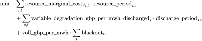
The single-node balance supplies demand and charging from available resources, storage discharge and recorded shortage:

Storage inventory records internal energy. charge_efficiency multiplies electricity absorbed from the grid, while delivered electricity is divided by discharge_efficiency:

Capacity bounds use period_hours to convert MW into period MWh:

Initial and terminal inventory determine net storage energy exchange across the horizon. The first transition starts from initial_soc_mwh. The default terminal_soc_rule = cyclic equates final and initial inventory; fixed uses terminal_soc_mwh_by_asset; free leaves final inventory within its bounds. With allow_blackout, shortage lies between zero and demand_mwh; otherwise its upper bound is zero. Defaults are period_hours = 0.5, voll_gbp_per_mwh = 17000 and zero degradation cost. The Study parameter market.voll_gbp_per_mwh accepts 0–1,000,000 GBP/MWh and enters the dispatch objective.
A second linear programme minimises storage throughput within the first solution's cost tolerance. primary.fun is the first-stage minimum in GBP; the second stage retains all physical constraints and adds

Both stages use HiGHS with primal and dual feasibility tolerances of  , and each requires a successful optimal termination before the calculation advances. The returned physical trajectory is
secondary.x. The maximum simultaneous charge and discharge, simultaneous, must be at most  MWh. Unused renewable energy is availability less accepted resource supply.
The demand-balance dual of the first optimum gives the marginal operating cost of period demand, displayed as “Balance shadow price”. Revenue multiplies the demand-balance dual in GBP/MWh by accepted MWh; storage earns the dual multiplied by discharge less charge. Consumer payment uses supplied demand. System cost adds annualised capital and the fixed operation and maintenance of non-wind, non-solar and non-storage assets to variable expenditure, degradation and shortage cost. The fixed-cost input is annual_fixed_opex_gbp; wind, solar and storage fixed operation and maintenance remains a memo line under Chapter 6.
PerfectForesightPSM.run(model_input):
    data = model_input.chronology
    validate_chronology(data, model_input.period_hours)
    _availability(...) and _marginal_costs(...): expand inputs to every period
    _layout(data): allocate resource, charge, discharge, soc and blackout
    assemble objective, throughput_objective, equality, rhs and bounds
    primary = linprog(objective, A_eq=equality, b_eq=rhs,
                      bounds=bounds, method="highs")
    primary_tolerance = max(1e-7, abs(primary.fun) * 1e-10)
    secondary = linprog(
        throughput_objective, A_ub=objective.reshape(1, -1),
        b_ub=[primary.fun + primary_tolerance], A_eq=equality, b_eq=rhs,
        bounds=bounds, method="highs")
    extract resource_period, charge_period and discharge_period
    extract soc_period and blackout
    check balance and simultaneous storage operation
    return costs and demand duals
Available run-of-river electricity
The natural-hydrology method derives available electricity from an inflow series and site parameters. run_of_river_dispatch reads HydroSite and CanonicalInflow; the default national PSM uses the statistical load factor and seasonal profile in Chapter 5.
A normalised electrical availability input scales installed power over the period. With inflow.unit = p.u., inflow.values lies in  ,
capacity_mw is MW and interval_hours is hours:

A water-volume input is converted through the site's turbine efficiency and MWh per water unit, then limited by electric power:

Accepted generation lies between zero and available; the default accepts all available electricity. curtailed is the remaining electrical potential. These arrays become available_energy_mwh, accepted_generation_mwh and curtailed_energy_mwh in the returned result. A 10 MW site over 0.5 h with factors  supplies
 MWh. This calculation operates independently in each period.
Conventional reservoir dispatch
A conventional reservoir allocates water across the complete inflow and electricity-value chronology to maximise generation value. reservoir_dispatch uses four period variables: turbine release q, ecological bypass, spill and end-period storage. All four use the declared water unit; the first three are volumes within the period. The conversion to electricity is

The linear programme minimises the negative value of generation plus a small spill penalty. energy_value_gbp_per_mwh is an externally supplied electricity-value series:

Water continuity links successive inventories and inflows. The first period starts from initial_volume:

Turbine, ordinary-release and ecological bounds restrict the use of water:

The ordinary-release bound and ecological minimum apply to turbine release plus bypass; spill enters water balance separately. A supplied terminal_volume fixes final inventory; otherwise final inventory remains within min_volume and max_volume. The parameter check requires maximum total release to be at least maximum turbine release and electricity from maximum turbine release to be at most turbine_capacity_mw multiplied by interval_hours, with tolerance  MWh.
The solver reads the complete inflow and value series and solves one SciPy/HiGHS linear programme. A successful solution returns water trajectories, generation and conservation residuals; objective_gbp is generation value less the spill penalty. An infeasible problem ends with the solver's failure result. The supplied inflow and electricity-value series determine the complete optimisation horizon.
reservoir_dispatch(parameters, inflow, *, energy_value_gbp_per_mwh):
    inflow.validate(); parameters.validate(inflow.interval_hours)
    conversion = (parameters.conversion_mwh_per_water_unit
                  * parameters.turbine_efficiency)
    allocate q, bypass, spill and storage for every period
    assemble objective, water equalities, release inequalities and bounds
    use parameters.terminal_volume as the final storage bound when supplied
    solved = linprog(objective, A_ub=inequalities, b_ub=upper,
                     A_eq=equalities, b_eq=rhs, bounds=bounds, method="highs")
    generation = q * conversion
    check previous + inflow.values[period] - q - bypass - spill - storage
    return generation, water trajectories and residuals
Hydrological input assembly
Natural-hydrology inputs comprise the site table, asset-to-site mapping, run-of-river inflow, reservoir inflow and reservoir parameters. Sites declare technology, capacity, turbine efficiency, bus, source and licence. Pumped storage uses the electrical-storage model. Each asset is assigned to a site, with mapping shares in ![(0,1]](/assets/methodology/math-en/eq-179.svg) and total shares per asset at most 1.
Inflow CSV files provide timezone-aware timestamps, interval length, site identifiers, values and water or electrical-availability units. The adapter requires finite nonnegative values, unique timestamps and consistent units; a supplied expected chronology is checked period by period. Site, mapping and parameter tables accept JSON or CSV. The declared missing-value treatment is none.
load_hydrology_inputs_from_pack joins the site, mapping, inflow and parameter tables by site_id; adapt_hydrology_csv preserves the declared interval and units. The independent function run_of_river_dispatch accepts site and inflow records and returns available_energy_mwh, accepted_generation_mwh and curtailed_energy_mwh, all in MWh. reservoir_dispatch accepts reservoir parameters, inflow and electricity values, returning generation_mwh in MWh and water trajectories in the declared water unit.
9 Carbon accounting parameters
VALUE calculates operational emissions and equipment-construction emissions separately before combining them under the selected accounting scenario. Operational emissions vary with generation and imported electricity, while construction emissions vary with installed capacity and the annualisation rule. The value_current_authoritative_v1 factor set supplies the accounting factors.
Generation and imported electricity
Operational emissions multiply generated or imported electricity by its selected factor. In build_operational_carbon_ledger, activity is the MWh read from generation_mwh_by_asset for each asset_id; kg is the factor converted to kg/MWh. Each emissions_tco2e entry records the resulting tonnes, and operational sums these entries:

The result is in tonnes, retaining the CO₂ or CO₂e definition of the selected factor. Zero values in the table refer to the direct operational generation boundary. Equipment-construction emissions are calculated using the capacity-based emissions factors in the next section. Import factors use fixed national averages or fallback values.
| Generation technology or import source | Factor kg/MWh | Gas basis | Data basis |
|---|---|---|---|
| Combined-cycle gas | 394 | CO₂ | NESO regional carbon-intensity methodology 2024 |
| Open-cycle gas | 651 | CO₂ | NESO regional carbon-intensity methodology 2024 |
| Biomass | 120 | CO₂e | NESO regional carbon-intensity methodology 2024 |
| Wind Solar Nuclear Conventional hydro Pumped hydro | 0 | CO₂ | NESO generation boundary |
| Imports from France | 53 | CO₂ | NESO fixed fallback factor |
| Imports from the Netherlands | 474 | CO₂ | NESO fixed fallback factor |
| Imports from Belgium | 179 | CO₂ | NESO fixed fallback factor |
| Imports from Ireland | 458 | CO₂ | NESO fixed fallback factor |
| Imports from Norway | 11.9 | CO₂e | NVE annual mean for physical electricity delivery in 2024 |
The source factors are converted to kg/MWh, with 1 g/kWh numerically equal to 1 kg/MWh. The original unit of Norway's factor is gCO₂e/kWh.
The biomass calculation uses the fixed factor of 120 kgCO₂e/MWh in the table. Its source reports an uncertainty range of ±120 gCO₂/kWh.
Construction emissions annualised by power capacity
Construction emissions are annualised for each operating asset. In _asset_embodied_lines, capacity_mw is operating power in MW and factor.value is its selected annual factor in tCO₂e/(MW·year). The per-asset value emissions becomes line.emissions_tco2e; embodied sums the construction entries:

Annual construction factors come from embodied_factors_desnz_unece.csv. Open-cycle gas uses the combined-cycle gas construction factor, and the electrolyser uses the proxy recorded in that table.
| Technology | Annual factor tCO₂e/(MW·year) |
|---|---|
| Solar | 38.544 |
| Onshore wind | 47.304 |
| Offshore wind | 96.1848 |
| Nuclear | 43.362 |
| Conventional hydro | 61.32 |
| Pumped hydro | 98.55 |
| Combined-cycle gas | 16.2936 |
| Open-cycle gas | 16.2936 |
| Biomass | 22.0752 |
| Electrolyser | 1.25 |
Storage emissions measured by energy capacity
Battery manufacturing emissions are annualised by rated energy capacity and equipment life. The selected factor is 89 kgCO₂e/kWh of capacity, the midpoint applied in the Longfield Solar Farm environmental statement of 2022. _asset_embodied_lines reads asset.energy_capacity_mwh in MWh and economic_life in years from economic_lifetime_years. Annual manufacturing emissions are

Hydrogen storage accounts separately for power equipment and energy storage. The energy-storage component uses a lifetime factor of 0.0006 tCO₂e/MWh of capacity, annualised over the asset's declared economic life. It is stored as ch4_h2_store_lifetime in factor_catalog.csv. The electrolyser power component uses the annual factor in the preceding section.
Carbon carried by stored electricity
Battery discharge enters storage_carried_transfer as a transfer of stored electricity, with zero additional operational emissions. Pumped hydro uses the zero operational factor in the table. Emissions from the charging source enter the generation or imported-electricity account. When storage_trace is supplied, a mixed-inventory calculation also tracks the emissions held in storage. Its inputs are period charge_mwh, discharge_mwh, charge_source_kgco2e_per_mwh and charge and discharge efficiencies.
The carbon inventory starts at zero. Charging adds emissions at the source intensity; discharging removes the fraction associated with the withdrawn inventory energy. In the calculation below, inventory_energy is in MWh and inventory_kg in kg; ending_inventory converts the closing carbon inventory to tonnes. Each period checks withdrawn against available inventory; an excess above  MWh terminates the calculation with
ValueError.
inventory_energy = 0.0
inventory_kg = 0.0
for charge, discharge, intensity in zip(
    storage_trace["charge_mwh"],
    storage_trace["discharge_mwh"],
    storage_trace["charge_source_kgco2e_per_mwh"]):
    admitted = charge * storage_trace["charge_efficiency"][0]
    inventory_energy += admitted
    inventory_kg += charge * intensity
    withdrawn = discharge / storage_trace["discharge_efficiency"][0]
    if withdrawn > inventory_energy + 1e-7:
        raise ValueError("Storage withdrawal exceeds available inventory")
    share = withdrawn / inventory_energy if inventory_energy > 0 else 0.0
    inventory_kg *= 1.0 - share
    inventory_energy -= withdrawn
ending_inventory = inventory_kg / 1000.0
Hydrogen-storage operation enters unresolved in the current ledger. _normalise_technology maps hydrogen_battery to hydrogen_storage, whose operational factor is empty; this activity makes operational and total return None. Hydrogen-storage construction emissions still use the power- and energy-capacity factors specified above.
Annual emissions and intensity
Annual emissions total sum operational emissions operational and annualised construction emissions embodied. Aggregation requires a matching factor for each activity and energy capacity and a positive economic life for storage. delivered_demand_mwh is served electricity; a positive value supplies the denominator for the following kg/MWh intensities:
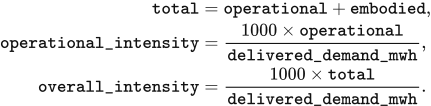
Construction emissions from line expansion
Line construction enters network_construction_embodied once in the commissioning year and is added to that year's total. adjust_carbon_ledger_for_network selects network assets with commissioning_year == year and status == "commissioned". For each selected asset, rating is MW, factor reads asset.embodied_carbon_factor_tco2e_per_mw in tCO₂e/MW, and emissions is tonnes:
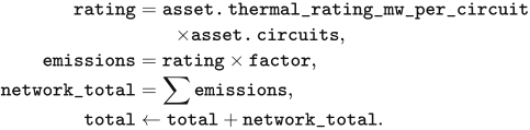
The updated total supplies overall_kgco2e_per_mwh and delivered_demand_kgco2e_per_mwh, using served electricity as denominator when it is positive. A selected line with a missing factor receives an unresolved construction entry and makes the total return None. The supplied fixed 23-zone network retains its declared branches; this additional calculation accompanies the optional line-expansion module.
Data and implementation
factor_catalog.csv stores the factors, units, accounting boundaries and source locations, while sources.csv stores source names. CarbonFactorDatabase reads value_carbon_factors.sqlite. build_operational_carbon_ledger connects dispatched electricity and operating assets to the selected factor set, and _asset_embodied_lines calculates annualised equipment-construction emissions.